Applying the TDS Technique to Identify and Analysis Wellbore Storage Effects

تطبيق تقنية التخليق المباشر (TDS) في تحديد وتحليل تأثير خزن البئر

Laila D. Saleh¹*, Abdussalam M. Mohamed¹, Mohammed H. Lagha¹, Moaid A. Alsagatti¹, Ahmed Y. Algizawi¹

DOI: https://doi.org/10.53796/hnsj73/13

Arabic Scientific Research Identifier: https://arsri.org/10000/73/13

Volume (7) Issue (3). Pages: 196 - 209

Received at: 2026-02-12 | Accepted at: 2026-02-19 | Published at: 2026-03-01

Download PDF

1. Introduction

Well testing of oil and gas wells is carried out by changing production rate before shutting in the well while recording pressure throughout the entire time of test. The two main objectives of testing an oil or gas well are; first to estimate reservoir parameters, such as permeability, skin factor and average reservoir pressure as well as to analyze reservoir behavior and define reservoir boundary limits [1].

A modern interpretation tool known as Tiab’s Direct Synthesis (TDS) technique which employs the pressure and pressure derivative curves to interpret pressure buildup and drawdown tests without using type-curve matching has been introduced by Tiab (1994 and 1995) [2, 3]. The TDS technique can be easily implemented for all kinds of conventional or unconventional systems. It can be easily applied on cases for which the other methods fail or are difficult to be applied. It is strongly based on the pressure derivative curve. The method works by sector or regions found on the test. This means once a given flow regime is identified, a straight line is drawn throughout it, and then, any arbitrary point on this line and the intersection with other lines as well are used into the appropriate equations for the calculation of reservoir parameters[2].

In some real field cases, conventional well test analysis technique face challenge when the radial flow region or wellbore storage regions are not observed on the pressure derivative plot TDS technique addressed this issue by analyzing specific, identifiable points on the derivative curve, which are then substituted into specialized equations .This approach enables the determination of reservoir parameters that would otherwise be unattainable in the absence of a clearly defined flow regimes.

The application case involving an absent radial flow region was examined in previous study [3]. This study aims to use the TDS technique, for determining the reservoir parameters and wellbore storage effect in case of wellbore storage line is not observed from pressure buildup tests for two oil wells from X field.

2. Methodology

TDS technique uses a log-log plot of pressure and pressure derivative data versus time to calculate various reservoirs and well parameters. In this technique, the values of the slopes, intersection points, and beginning and ending times of various straight lines from the log-log plot can be used in exact analytical equations to calculate different parameters as it is shown in the following.

CASE 1: unit-slope and infinite-acting line are observed; (Fig.1) illustrate this case.

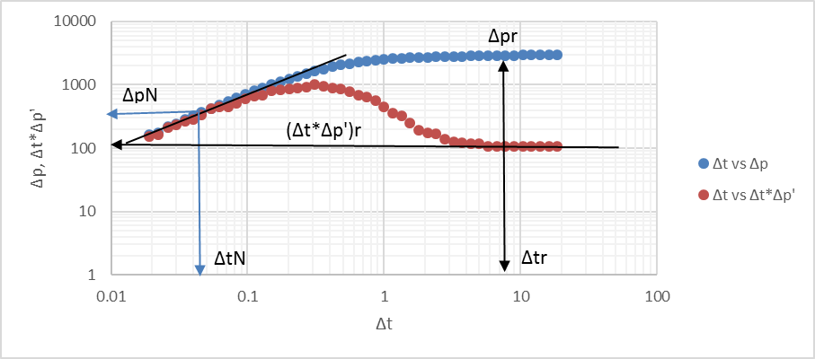
Figure (1): Unit-slope and infinite-acting line are observed

• Wellbore storage effect:

Wellbore storage is after flow of fluids into the wellbore after the well is shut-in at the wellhead. During wellbore storage, reservoir effects are masked or distorted, making it impossible to quantify well properties such as permeability, skin and P*. In this case the wellbore storage effect can be calculated from the following equation:

…………………………………………. (1)

The permeability can be determined using infinite acting radial flow line data by using the following equation:

…………………………………………. (2)

The skin factor can be calculated from radial flow pressure and pressure derivative data by using the following equation:

……………………………. (3)

Pressure loss or gain due to skin calculated by following equation:

…………………………………. (4)

For a well in the center of a circular reservoir, the average reservoir pressure is obtained from a log‐log plot of pressure and pressure derivative versus time according to the following expression:

…. (5)

the Flow Efficiency can be determined by using the following equation:

…………………………………. (6)

The Productivity index can be determined by using the following equations:

………………………………. (7)

………………………. (8)

CASE 2: the unit-slope line is not observed (no wellbore storage), (Fig.2) illustrate this case.

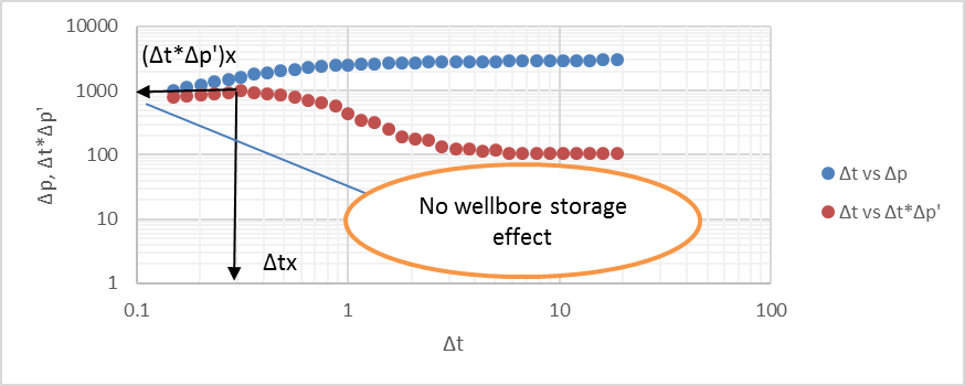
Figure (2): The unit-slope line is not observed (no wellbore storage)

In this case the wellbore storage effect ”C “ cannot be calculated from equation (1) because absent points in unite slope line ( and ), therefore, the following equation can be used:

………………………. (9)

In case of unit-slope line and Hump (peak) are not observed the effect of wellbore storage can be obtained by estimating time start radial flow () and using following equations:

………………………………. (10)

……………………. (11)

(Fig.3) illustrate the case of unit-slope line and Hump (peak) are not observed.

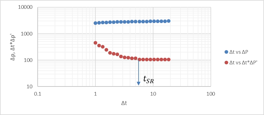
Figure (3): Unit-slope line and Hump (peak) are not observed

• Boundary effects in diagnostic plots

Reservoir boundaries have significant influences on the shape of the diagnostic plot. The effects of boundaries appear following the middle-time region (infinite-acting radial flow) in a test.

• Well in an infinite-acting reservoir:

An infinite acting reservoir is a reservoir without any boundaries, therefore boundary effects will not appear on the analysis plots during the duration of the test.

• Constant Pressure Boundary:

A constant pressure boundary is a boundary that provides pressure support. This kind of boundary usually occurs in reservoirs with aquifer support. Steady state flow signifies that a constant pressure boundary has been reached.

• No-Flow Boundary:

A no-flow boundary is a boundary that does not allow flow through it. This kind of boundary usually occurs in reservoirs with sealing faults or is created between producing wells that are equally spaced and producing at the same rate. Pseudo-steady state flow signifies that all no-flow boundaries have been reached, (Fig.4) illustrates sealing faults cases.

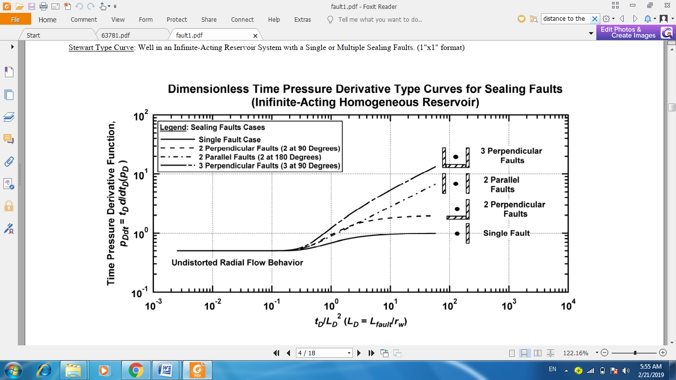
Figure (4): Sealing faults cases ^[9].

• Distance to Boundary

The distance to the boundary is the distance between the well and the boundary. The boundary may be a no flow or constant pressure boundary.

TDS technique can be used to calculate the distance from well to fault by estimating the time at which radial flow regime ends (), and then using the following equation:

………………………………. (12)

3. Field case

This study includes using TDS technique on MS Excel software to analysis well test data to calculate wellbore storage effect in two cases (complete test and test without unit slope line), and other properties such as permeability, skin factor, average reservoir pressure, for two wells (H1& H2), which are located in X oilfield in Libya .

3.1 Reservoir Properties

Data from numerous plug analyses shows that the reservoir properties do not vary significantly across the field. Porosities typically range from 10 – 15%. The effective permeability to oil ranges between 150 and 300 mD, although individual wells show values of up to 1300 mD (PRC 1990), which is obviously related to a certain degree of fractures in the reservoir (BERNHARD, GRUENWALD 1998). The net / gross ratio varies between 0.8 and 0.98.

3.2 Analyses of Well H1

Well H1 is located in the western part of X field, it was spud on 11Jun2006 and completed on 21Aug 2006, Initial OWC was found at 12328ft-md-BDF while secondary OWC was encountered at 12258ft –md –BDF.

The well found a net pay of 583ft of reservoir in the main oil zone of the Upper Gargaf Fm with an average porosity of 11.5% and 6.1% water saturation.

3.2.1 TDS Technique

TDS Technique used to analysis this well in two cases as following:

• The unit slope line is observed (complete test).

Step (1): Prepare General Data Required for the Analysis. Table (1) introduces the required reservoir data

Table (1): Input data for well H1

STB/day	4087
Hr	33.585
bbl/STB	1.6
Cp	0.6
Psia-1	2.06
Ft	460
Ft	0.013283
Ft	583
–	0.115	ɸ

Step (2): plot pressure versus time. (Fig.5) illustrate the change in pressure with time before and during the shut-in period for well H1.

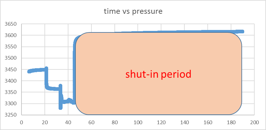
Figure (5): Pressure vs time for well H1

Step (3): Plot ΔP and ∆t×ΔP’ versus time on a log-log graph and Δt versus Δp on semi log graph for shut-in period. (Fig.6 & 7) shows ΔP and ∆t×ΔP’ vs time and Δt vs Δp respectively for well H1.

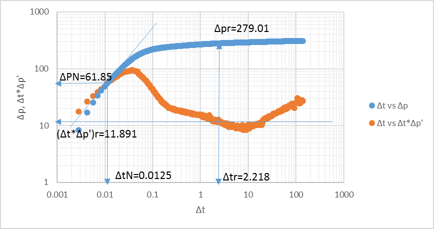
Figure (6): Pressure drop and pressure derivative vs time for well H1

The unit slop line that used to calculate wellbore storage effect illustrated in this case (complete test), also the mid and late time regions are observed.

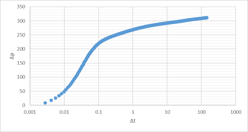
Figure (7): Pressure drop vs time for well H1

Step (4): Draw the infinite-acting radial flow line. This line is of course horizontal. Read the value . As shown in (Fig.6).

Step (5): Select any convenient time during infinite-acting radial flow line and read from the pressure curve. As shown in (Fig.6).

Step (6): Draw the unit-slope line corresponding to the wellbore storage flow regime using early-time pressure and pressure derivative points. Read the coordinates of a point N on the unit-slope line: and . As shown in (Fig.6).

Step (7): Calculate the WBS coefficient from Eq. (1)

Step (8): Calculate the permeability from Eq. (2)

The permeability of this well is good.

Step (9): Calculate the skin factor from Eq. (3)

In this case the value of skin factor mainly means that the well had a damage.

Step (10): Calculate pressure drop due to skin effect by using eq. (4)

Step (11): Select any convenient point from the late time data exhibited on the pseudo steady state flow line and read (∆P)_pss = 309.54 and (∆t*∆P’)_pss = 30.572 respectively, and calculate average reservoir pressure from eq. (5). The last pressure value, that is 3616.21 psi, is taken as P_i.

Step (12): calculate flow efficiency from eq. (6).

Step (13): calculate actual and theoretical Productivity Index from Eq. (7) and Eq. (8) respectively.

The actual and theoretical productivity values are almost the same this indicates that the test analysis was good.

Step (14): calculate the distance from well to fault by using Eq. (12).

• The unit slope line is not observed.

in this case the wellbore storage effect can be calculated by determining the coordinates of the maximum point (peak) on the ∆t*∆p’ versus time curve, i.e. ∆t_x and (∆t*∆p’)_x, As shown in (Fig.8),.and then using eq. (9)

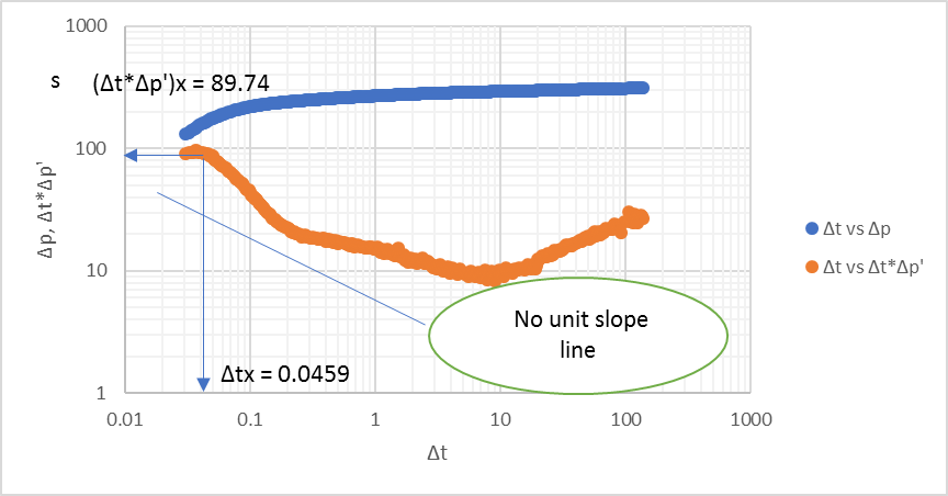
Figure (8) : Pressure drop and pressure derivative vs time for well H1

The value of wellbore storage effect obtained by Using the advantage of TDS technique (points from peak zone) gave a good result and approximately similar to that obtained in the case of unit slope line is observed.

 

3.3 Analyses of Well H2

Well H2 is proposed as s development well in the Upper Gargaf sandstone of the X Oil Field.

The well was perforated by using TCP gun, HMX, 6shots/ft, 60° Phasing, 2.88″ OD Omega Powerjet 2906. The perforation intervals from 11481’ to 12110’ md-bdf The initial Oil-Water Contact at 12,389 ft-md-bdf, secondary Oil-Water Contact at 12,260 ft-md-bdf, and reference depth is 12,150 ft-TVDSS.

The well was brought on stream on 30th November 2009 and test run from 26th December 2009 to 2nd January 2010. Test production rates vary from 2245 bopd to 5192 bopd (36/64” to 64/64”) with a 0.2 – 0.3 % water cut and without gas-lift.

3.3.1 TDS Technique

TDS Technique used to analysis this well in two cases as following:

• The unit slope line is observed (complete test).

Step (1): Prepare General Data Required for the Analysis. Table (2) introduces the required reservoir data

Table (2): Input data for well H2

STB/day	5192
Hr	67.502
bbl/STB	1.499
Cp	0.38
Psia-1	1.708
Ft	300
Ft	0.25
Ft	792
–	0.129	ɸ

Step (2): plot pressure versus time. (Fig.9) illustrate the change in pressure with time before and during the shut-in period for well H2.

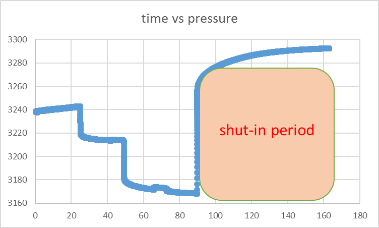
Figure (9): Pressure vs time for well H2

Step (3): Plot ΔP and ∆t×ΔP’ versus time on a log-log graph and Δt versus Δp on semi log graph for shut-in period. (Fig.10).and (Fig.11).shows ΔP and ∆t×ΔP’ vs time and Δt vs Δp respectively for well H2.

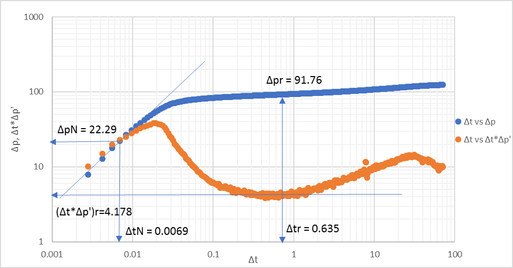
Figure (10): Pressure drop and pressure derivative vs time for well H2

The unit slop line that used to calculate wellbore storage effect illustrated in this case (complete test), also the mid and late time regions are observed.

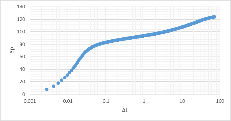
Figure (11): Pressure drop vs time for well H2

Step (4): Draw the infinite-acting radial flow line. This line is of course horizontal. Read the value . As shown in (Fig.10).

Step (5): Select any convenient time during infinite-acting radial flow line and read from the pressure curve. As shown in (Fig.10).

Step (6): Draw the unit-slope line corresponding to the wellbore storage flow regime using early-time pressure and pressure derivative points. Read the coordinates of a point N on the unit-slope line: and . As shown in (Fig.10).

Step (7): Calculate the WBS coefficient from Eq. (1)

Step (8): Calculate the permeability from Eq. (2)

The permeability resulted in this well is good.

Step (9): Calculate the skin factor from Eq. (3)

In this case the value of skin factor mainly means that the well had a damage.

Step (10): Calculate pressure drop due to skin effect by using eq. (4)

Step (11): Select any convenient point from the late time data exhibited on the pseudo steady state flow line and read (∆P)_pss =117.06 and (∆t*∆P’)_pss = 14.239 respectively, and calculate average reservoir pressure from eq. (5). The last pressure value, that is 3292.44 psi, is taken as P_i.

Step (12): calculate flow efficiency from eq. (6).

Step (13): calculate actual and theoretical Productivity Index from Eq. (7) and Eq. (8) respectively.

In this case, The actual and theoretical productivity values are not the same, and the reason may be due to uncertainty in average pressure value.

Step (14): calculate the distance from well to fault by using Eq. (12).

• The unit slope line is not observed.

In this case, the wellbore storage effect can be calculated by determining the coordinates of the maximum point (peak) on the ∆t*∆p’ versus time curve, i.e. ∆t_x and (∆t*∆p’)_x, As shown in (Fig.12)., and then using eq. (9)

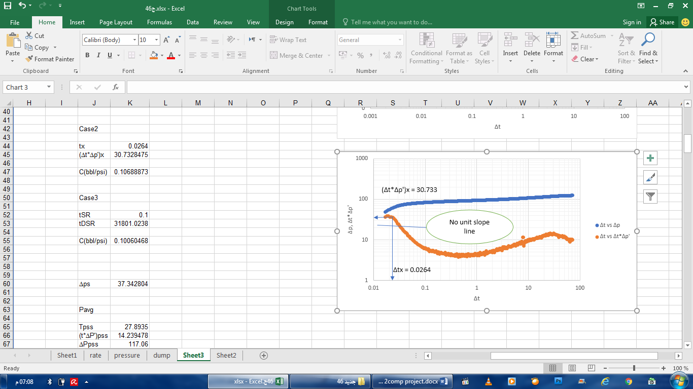
Figure (12): Pressure drop and pressure derivative vs time for well H2

The value of wellbore storage effect obtained by using the advantage of TDS technique (points from peak zone) gave a good result and approximately close to that obtained in the case of unit slope line is observed.

 

The results were compared with the results from KAPPA software as shown in Table (3).

Table (3) : Summary of the results

Wells#	parameters	TDS		KAPPA
		Complete test	Test without unit slope line
H1	C (bbl/psi)	0.055	0.054	0.05
	K (md)	39.957	–	40.264
	S	2.152	–	2.2
	ΔPskin (psi)	51.171	–	51.924
	(psi)	3585.316	–	3585.91
H2	C (bbl/psi)	0.1	0.106	0.09
	K (md)	63.106	–	63.667
	S	4.469	–	4.5
	ΔPskin (psi)	37.343	–	37.269
	(psi)	3279.932	–	3258.24

4. Conclusion

• TDS technique is particularly useful when the early-time unit slope line is not observed due to the lack of points or sever noise problem.
• In wells H1and H2 taking the coordinate points (, ) after maximum point of peak to give more accurate results.
• Another advantage of TDS technique that the wellbore storage effect can be estimating in the absent of the early time unite slope line and the hump.

References

1. Tarek Ahmed, 2010. “Reservoir Engineering Handbook”, 4th edition .
2. Tiab, D., 1994. “Analysis of Pressure and Pressure Derivative without Matching: Vertically Fractured Wells in Closed Systems,” Journal of Petroleum Science and Engineering 11, 323.
3. Tiab D., 1995. “Analysis of pressure and pressure derivative without type-curve matching: skin and wellbore storage”. J Pet Sci Eng.
4. Saleh, L., Traki, A., Alhaj, H., Gergab, M., Al-Osta, M., 2025 “Well Test Interpretation with TDS Technique: Detection and Absence of Infinite Acting Radial Flow, Case Study” Alqalam Journal of Science, 207-216