Solving Linear Systems with non-integer coefficients by using some soft ware

Dr. Abbas Abdelaziz Gumma Mahmoud¹

DOI: https://doi.org/10.53796/hnsj65/14

Arabic Scientific Research Identifier: https://arsri.org/10000/65/14

Volume (6) Issue (5). Pages: 157 - 165

Received at: 2025-04-07 | Accepted at: 2025-04-15 | Published at: 2025-05-01

Download PDF

.

1. Introduction: In this paper we will try to take advantage of the great development in the field of software to employ them in the direction of building mathematical models and resolution.

The aims look for optimization programs to solve systems of linear equations and so these methods requiring less mathematical skills and effort mentally contributes to less than reliable in various applications for non-specialists in mathematics. And then compare this software to find the difference between them and the errors if it is exist. The study helps to shorten the time in the solution of linear systems using some ready-made software with less effort and small errors. Also through the study note that can non-professionals in the field of mathematics to deal with linear systems.

2. Study goal:

The present study aims to look for optimization programs to solve systems of linear equations and so these methods requiring less mathematical skills and effort mentally contributes to less than reliable in various applications for non-specialists in mathematics. And then compare this software to find the difference between them and the errors if it is exist.

3. The problem of the study:

Study the problem lies in the difficulty of solving systems of linear equations by standard methods so to find the exact solutions to these systems using ready-made software.

4. The importance of the study:

The study helps to shorten the time in the solution of linear systems using some ready-made software with less effort and small errors. Also through the study note that can non-professionals in the field of mathematics to deal with linear systems.

5. Case study :

In this case the coefficients of the variables are non-integer

9.9 x₁ – 1.5 x₂ + 2.6 x₃ = 0

0.4 x₁ + 13.6 x₂ -4.2 x₃ = 8.2

0.7 x₁ + 0.4 x₂ + 7.1 x₃ = -1.3

Solution of Case Study 2 manually by Iterative Method:

Reduce the system to the normal form:

9.9 x₁ = 1.5 x₂ – 2.6 x₃

13.6 x₂ = 8.2 – 0.4 x₁ + 4.2 x₃

7.1 x₃ = -1.3 – 0.7 x₁ – 0.4 x₂

Or

x1 = x2 – x3

x2 = – x1 + x3

x3 = – x1 – x2

 = ,

Then write the system in the form

x = +  x

zero approximation:

x =

or:

=

First approximation:

= + x =

Second approximation:

= + x =

Third approximation:

= + x =

Forth approximation:

= + x =

The following Table(1) shows the answers of case study 2 by

Approximation method (Iterative Method):

Table (1)

Approximation Method Answers

Variable	Value
X1	0.1397
X2	0.5288
X3	-0.2267

Table (2) shows the verifying of the solutions.

Table (2)

verification of Approximation Method

Equation	Constant	Substitution Value	The error
Equation 1	0	0.0004099999999	-0.00040999999999
Equation 2	8.2	8.1997	0.000299999999997
Equation 3	-1.3	-1.30026	0.000259999999999

4.Solution of Case by using Excel Solver:

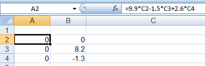
As shown in Figure (1), enter the system

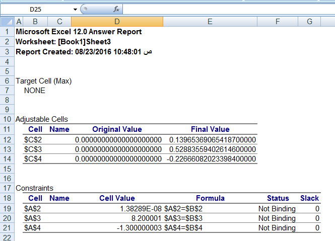Then the solution shows like in Figure (2).

Figure (2): Excel Answer

The following Table (3) shows the answers of case by

Excel Solver.

Table (3)

Answers of Excel

Variable	Value
X1	0.139653690654187
X2	0.528835594026146
X3	-0.226660820233984

Table (4) shows the verifying of the solutions.

Table (4)

verification of Excel

Equation	Constant	Substitution Value	The error
Equation 1	0	1.38 x 10-08	-0.0000000138289
Equation 2	8.2	8.200001	-0.0000001
Equation 3	-1.3	-1.3	0

5. Solution of Case by using Lindo:

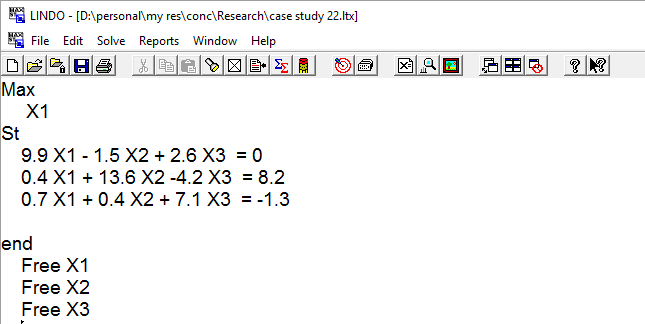Figure (3) shows the entry of the Case :

Figure (3): Lindo input

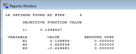Then the solution appear as shows in Figure (4).

Figure(4): Lindo Answer

The following Table (5) shows the answers of case by Lindo

Table (5)

Answers of Lindo

Variable	Value
X1	0.139654
X2	0.528836
X3	-0.226661

Table (6) shows the verifying of the solutions of Case using Lindo.

Table (6)

Case verification of Lindo solution

Equation	Constant	Substitution Value	The error
Equation 1	0	0.000002	-0.000002
Equation 2	8.2	8.2000074	-0.0000074
Equation 3	-1.3	-1.3000009	0.00000089999999989

6. Solution of Case Study using Maxima:

Enter the system as seen in Figure (5)

Figure (5): Maxima input

Figure (6): Maxima Answers

Then the solution appears as Figure (6)

The following Table (7) shows the answers of case study 2 using

Maxima.

Table (7)

Answers of Maxima

Variable	Value
X1	0.13965367693931500000
X2	0.52883552267193300000
X3	-0.22666081449666100000

Table (8) shows the verifying of the solutions of Case using maxima.

Table (8)

verification of Maxima solution

Equation	Constant	Substitution Value	The error
Equation 1	0	0	0
Equation 2	8.2	8.19999999999999	0.000000000000001
Equation 3	-1.3	-1.3	0

6. Solution of Case Study by using SimSolve :

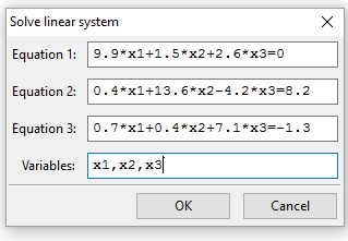
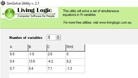Figure (7) shows the input of the system in SimSolve

Figure (7): SimSolve input

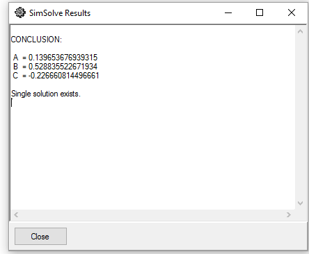Then the solution shows as Figure (8)

Figure (8): SimSolve Answers

The following Table (9) shows the answers by using SimSolve.

Table (9)

Answers of SimSolve

Variable	Value
X1	0.139653676939315
X2	0.528835522671934
X3	-0.226660814496661

Table (10) shows the verifying of the solutions of Case 2 using SimSolve.

Table (10)

verification of SimSolve solution

Equation	Constant	Substitution Value	The error
Equation 1	0	0	0
Equation 2	8.2	8.2	0
Equation 3	-1.3	-1.3	0

 

7. Conclusion : The case study involved a written system contained
a non-integer coefficient to note the differences in accuracy of solutions.
In this case identical solutions of all systems up to 10-6

In the case sudy represents a sample of:

non-integer coefficients, and thus may produce solutions not identical values. This case recorded the following :

	Error
	Iterative Method	Excel Solver	LINDO 6.1	MATLAB	Maxima	SimSolve
Equation1	-0.000409	0.00000001	-0.000002	-0.000409	0	0
Equation2	0.0002999	-0.0000001	-0.000007	0.0002999	0	0
Equation3	0.0002599	0	0.00000089	0.0002599	0	0
Avg	0.000322	0	0.000003	0.000322	0	0

Avg = (∑ Error )/number of Errors

• All the software in the match results untill 10^-5 , exept MATLAB match untill 10^-3 .
• MATLAB sofware and Sidel Method (manully) gives same solution .
• Since SimSolve uses one of the methods of elimation (Gauss-Jordan) so there are no errors in the solution to the lack of non-zero values in the coefficients matrix.

By offering a solution in the Maxima it appeared to be running one of the iterative methods, which repeats and substitute until error is belong to zero. So nonexisting error.

References

1.A. Barry (2003). Computational methods in O.R using Lindo and Lingo (2003). Available at: http://www.abarry.ws/books/CalculationMethodsBook.pdf/

2.Bosch, W. W., and Strickland, J. (1998). Systems of linear equations on a spreadsheet. Mathematics & Computer Education, 32, (1), 11-16.

3.Camporesi, Roberto (2016). A Fresh Look at Linear Ordinary Differential Equations with Constant Coefficients. Revisiting the Impulsive Response Method Using Factorization. International Journal of Mathematical Education in Science and Technology, v47 n1 p82-99 2016.

4.Carley, Holly (2014). On Solving Systems of Equations by Successive Reduction Using 2×2 Matrices. Australian Senior Mathematics Journal, v28 n1 p43-56 2014.

5.Deane Arganbright (n. d). Innovative Uses of Excel in Linear Algebra. Department of Mathematics and Computing Science Divine Word University, Papua New Guinea. Available online at: http://atcm. mathandtech. org/EP2011 /regular _papers / 3272011_19192.pdf

6.Edwards, Thomas G.; Chelst, Kenneth R.; Principato, Angela M. and Wilhelm, Thad L. (2015). Investigating Integer Restrictions in Linear Programming. Mathematics Teacher, v109 n2 p136-142 Sep 2015.

7.El-Gebeily, M. and Yushau, B. (2008). Linear System of Equations, Matrix Inversion, and Linear Programming Using MS Excel. International Journal of Mathematical Education in Science and Technology, 39(1), 83-94.

8.Greg Harvey (2007). Microsoft Office Excel 2007: All-in-one desk reference .Wiley Publishing, Inc.

9.Jerome, Lawrence (2012). Generalized assignment matrix methodology in linear programming. International Journal for Technology in Mathematics Education, v19 n1 p25-41 2012.

10.LINDO User’s Manual (2003). LINDO SYSTEMS INC. Available online at: http://www.lindo.com.

11.Macsyma system (2001). Maxima User Manual.

12.Martin Golubitsky and Michal Dellnitz (1999). Linear algebra & differential equations using MATLAB. An International Thomson Publisher Company.

13.Mike Brookers (2011). The Matrix Reference Manual. Imperial College – London.

14.N. I. Danilina, N. S. Dubrovskaya, O. P. Kvasha and G. L. Samirov (1988). Computational Mathematics. Mir Publisher.

15.O. V. Manturov and N. M. Matveev (1989). A Course of Higher Mathematics. Mir Publisher.

16.R. L. Burden and J. D. Faires (2011). Numerical Analysis (9^th ed.).Youngstown State University.

17.Roanes-Lozano, Eugenio (2011). Some applications of algebraic system solving. International Journal for Technology in Mathematics Education; 2011, Vol. 18 Issue 3, p149.

18.Stephen Moffat (2011). Excel 2010 Part II. Stephen Moffat & bookboon.com Available online at: http //www.bookboon.com.