Comparative Study of Three Methods of penalized Quantile regression based on EMD for improving the Accuracy of the Model Selection

دراسة مقارنة لثلاث طرائق للانحدار الكمي المُعاقَب المعتمدة على تحليل الأنماط التجريبية (EMD) لتحسين دقّة اختيار النموذج

Ali Ambark¹, Mahdi Madhi¹, Mohd Tahir Ismail²

DOI: https://doi.org/10.53796/hnsj71/22

Arabic Scientific Research Identifier: https://arsri.org/10000/71/22

Volume (7) Issue (1). Pages: 364 - 376

Received at: 2025-11-10 | Accepted at: 2025-12-17 | Published at: 2026-01-01

Download PDF

1. Introduction

In both natural and artificial systems, time series processes are often used to represent variables of interest; these are often non-stationary and non-linear (Masselot et al., 2018). Analysing such data requires addressing the important issue of decomposing these non-stationary and non-linear time series. Despite a lack of analytical methods (Huang, 2005), techniques like the Fourier transform (Titchmarsh, 1948), the Wigner distribution (Classen & Mecklenbrauker, 1980), and wavelet analysis (Chan, 1995) have been applied to time series. The empirical mode decomposition (EMD), introduced by (Huang et al., 1998), offers an intuitive and adaptive method for decomposing nonlinear and nonstationary time series data. As the initial step in the Hilbert-Huang transform (HHT), EMD contrasts with traditional methods like wavelet decomposition and Fourier decomposition by imposing no prior assumptions on the data, allowing for data-driven decomposition into distinct oscillatory components. Although empirically derived and lacking a formal mathematical basis, EMD effectively separates a data series into components associated with specific oscillation frequencies.

Mean regression analysis (most commonly ordinary least squares regression, OLS) is one of the most widely used statistical methods. Despite its desirable properties like linearity and unbiasedness, its reliance on the mean of the response variable makes it vulnerable to heavy-tailed error distributions and outliers. Quantile regression, introduced by (Koenker & Bassett, 1978), has emerged as a robust alternative, gaining popularity for its ability to model the relationship between response and predictor variables at any quantile of the conditional distribution. Unlike mean regression, quantile regression makes no distributional assumptions about the error term, provides a comprehensive view of the relationship across the entire conditional distribution (Koenker & Bassett, 1978), and is robust to outliers and heteroscedasticity. These advantages have led to its widespread adoption in practical applications. By quantifying the entire conditional distribution, quantile regression offers an overall assessment of predictor effects at various response quantiles (Koenker, 2005). However, multicollinearity, arising from dependence among predictor variables, remains a significant challenge in regression analysis, leading to inflated sample variance and inaccurate signals in regression coefficients, thereby affecting both inference and estimation (Ali et al., 2019).

Variable selection is crucial for identifying key predictors from a large set, leading to simpler models with improved prediction accuracy. Regularized regression techniques, which simultaneously select variables and estimate coefficients by penalizing the objective function, are essential for this purpose (Khan et al., 2019). These techniques include ridge regression (Hoerl & Kennard, 1970), LASSO (Tibshirani, 1996), and elastic net (Zou & Hastie, 2005), which combines ridge and LASSO penalties.

Moreover, penalized methods have found success in quantile regression. For instance, (Xu et al., 2017) and (Li & Zhu, 2008) employed L1 penalized quantile regression using the LASSO penalty, while (Burgette et al., 2011) used LASSO and elastic net penalties to identify key predictors. (Zaikarina et al., 2016) and (Sadig & Bager, 2018) applied LASSO and ridge penalties to address multicollinearity, with (Zaikarina et al., 2016) using modified percentile cross-validation. (Yan & Song, 2019) explored penalized quantile regression with elastic net and adaptive elastic net penalties. Under a Bayesian framework, (Alhamzawi et al., 2012) and (Alshaybawee et al., 2017) proposed Bayesian estimation approaches using adaptive LASSO quantile regression. Furthermore, empirical mode decomposition (EMD) has been integrated into quantile regression, as demonstrated by (Jaber et al., 2014) combining EMD with local polynomial quantile regression, (Zhang et al., 2020) employed EMD to reduce noise in wind speed series for probability density forecasting using QR and KDE. (Ambark & Tahir Ismail, 2024) studied penalized quantile regression based on EMD to address the problem of multicollinearity and perform variable selection and accurate prediction. (Ambark et al., 2023) presented elastic net penalized quantile regression based on the EMD for selecting decomposed components that exhibit the most potent effects on the response variable, and multicollinearity between the decomposition components was dealt with.

This paper is devoted to the comparison of three methods, which are EMD-LQR, EMD-RQR, and EMD-EnetQR in the literature. This comparison aims to identify the best methods, which are dealing with the heterogeneity, and to improve the accuracy of model selection by selecting the predictors that have the most effect on the response variable.

The rest of this paper is organized as follows. In Section 2, we give a description of the EMD method, quantile regression, and penalized quantile regression. Section 3 simulation studies are carried out to compare the performance of the three methods. Section 4 shows the real examples. Section 6 presents some conclusions and gives some discussion.

1. Methodology

In this section, we briefly describe the applied methods. Firstly, the EMD technique which deals with non-stationary and non-linear datasets by the sifting process. Secondly, quantile regression which deals with heterogeneity problems. Finally, penalized quantile regression which including Ridge, Lasso, and Elastic Net regression for variable selection.

• 1. Empirical Mode Decomposition (EMD)

Empirical mode decomposition (EMD), developed by (Huang et al., 1998), for decomposes nonlinear and non-stationary time series datasets into intrinsic mode functions (IMFs) and a residual through a sifting process. This unsupervised data-driven decomposition requires no prior information. Each IMF must satisfy two conditions:

(1) The number of local extrema and zero-crossings must be equal or differ by one.

(2) The mean of the envelopes defined by local maxima and minima must be zero at any given time point. The EMD process can be expressed as follows:

The original signal is decomposed into intrinsic mode functions (IMFs) denoted by , and a residue . This decomposition is achieved through the Empirical Mode Decomposition (EMD) algorithm, which employs an iterative sifting process to separate the IMFs and residual. Notably, IMFs possess physical definitions for instantaneous frequency and amplitude, providing a physically meaningful time-frequency-energy representation of the time series. The sifting process procedure includes the following steps:

1. Using the original signal for the sifting process on the assumption that the value of the two repetition indicators is .
2. Identify all local extrema, including minima and maxima.
3. Construct envelopes: Connect all the minima and maxima with a cubic spline line to generate the lower and upper envelopes.
4. Compute the local mean of the upper and lower envelope by using Equation 6.
5. Subtract the mean envelope m(t) from the original signal X(t) to obtain the first component IMF
6. Check whether is an IMF or not, according to IMF conditions.

If not, replace with , increment the iteration indicator , and repeat the sifting process (steps 2-5) until satisfies the IMF conditions.

If satisfies the IMF definition, then = ; save and proceed to step 7.

1. Calculate the residual r(t) as the formula:

Check if the residue function is monotonic, constant, or satisfies the standard deviation stopping criterion. which needs the normalized squared difference between two successive sifting operations to be small. The difference is defined as follows:

Save the residue and all intrinsic mode functions (IMFs), then stop the sifting process.

Otherwise, if the residue is not monotonic or constant, replace the with and repeat the sifting process until the residue is monotonic, constant, or satisfies the stopping criterion.

The Empirical Mode Decomposition (EMD) method decomposes a complex signal into a small number of intrinsic mode functions (IMFs), ordered from high to low frequencies, based on local characteristic scales (the distance between successive local extrema). Each IMF has symmetric upper and lower envelopes, with the number of zero-crossings and extremes differing by at most one. IMFs represent oscillatory scales within a narrow spectrum and are typically considered quasi-stationary. For example, an IMF derived from a three-month economic time series can represent the seasonal component.

• 1. Quantile Regression

Quantile regression (QR) (Koenker & Bassett, 1978) is a robust method for modeling the conditional quantile function. Unlike traditional regression, QR is resistant to outliers and effectively handles data heterogeneity. By examining different quantile levels, it offers a nuanced understanding of the relationship between the response variable and predictor variables, making it widely applicable across scientific fields.

Consider the linear regression model given by

where represents the value of the response variable vector for the observation, represents the vector of p predictor variables from the design matrix , excluding the intercept, denotes the regression model parameters that must be estimated, denotes the value of the random error term. Suppose that the linear quantile regression model is following

The τ th conditional quantile function can then be estimated by solving the following optimization problem (Davino et al., 2014):

(8)

is the check loss function defined as follows:

(9)

or equivalently .

To improve quantile regression and regularization, a penalty function is added to equation (9), as follows:

where is the tuning parameter and is the penalty function.

To implement the comparison, estimating the tuning parameter λ is crucial in that it regulates model complexity. A small value of λ leads to increased model variance by including many variables, while a large λ oversimplifies the model, increasing bias. Therefore, selecting the optimal λ is important. Common methods include cross-validation (CV) (Stone, 1974), Akaike’s Information Criterion (AIC) (Akaike, 1973), and the Bayesian Information Criterion (BIC) (Schwarz, 2007).

• 1. Penalized Quantile Regression

This section discusses QR variable selection. We specifically demonstrate variable selection utilizing ridge regression (Hoerl & Kennard, 1970), LASSO regression (Tibshirani, 1996), and elastic net regression (Zou & Hastie, 2005) in a QR scenario.

• • 1. Ridge Penalized Quantile Regression

Ridge regression proposed by (Hoerl & Kennard, 1970), is a widely applied technique that minimizes the residual sum of squares subject to a constraint on the coefficients. As a continuous shrinkage method, it improves prediction accuracy by balancing bias and variance and is commonly used to address multicollinearity. The ridge estimator is given as follows:

where λ is the penalty parameter in the range 0 < λ < 1 and is the -norm of the vector . We consider Ridge penalized quantile regression based on EMD denoted by RQR.EMD. The ridge penalized quantile regression is used as the following formula:

• • 1. LASSO Penalized Quantile Regression

LASSO (Least Absolute Shrinkage and Selection Operator), introduced by (Tibshirani, 1996), is a regression technique used in generalized linear models for predictor selection. It achieves this by shrinking some coefficients to zero, effectively imposing a constraint on the regression coefficients. LASSO minimizes the residual sum of squares subject to the constraint that the sum of the absolute values of the coefficients is below a constant. The LASSO estimate is given as follows:

Where s ≥ 0 is a tuning parameter, and is the -norm of the vector . An equivalent formulation of LASSO is to solve the penalized likelihood problem as follows.

LASSO quantile regression is a regularization method that performs simultaneous estimation and variable selection. We consider LASSO penalized quantile regression based on EMD denoted by LQR.EMD. The LASSO quantile regression estimates are defined as (Li & Zhu, 2008).

• • 1. Elastic Net Penalized Quantile Regression

(Zou & Hastie, 2005) introduced Elastic Net regularization, a convex combination of LASSO and Ridge penalties, to estimate coefficients by minimizing the regression loss function with an Elastic Net penalty.

The Enet estimator is given as follows:

Where , are tuning parameters , , λ1 and λ2 are dependent on dataset and automatically selected via cross-validation (Al-Jawarneh et al., 2024; Masselot et al., 2018; Melkumova & Shatskikh, 2017; Zou & Hastie, 2005). The optimal tuning parameters λ1 and λ2 minimize the mean squared error (MSE) (Friedman et al., 2010).

Equation (15) can be rewritten as follows by substituting and and becomes equivalent.

where is a regularization parameter . when , the Enet estimation undergoes the Ridge estimator, whereas when α = 1, the Enet estimation is subject to the LASSO estimator. We consider LASSO penalized quantile regression based on EMD denoted by EnetQR.EMD

The elastic-net penalized quantile regression is used as the following formula:

1. Application

In this section, we implemented the numerical simulation experiment and a real data application to compare three previously described methods. This analysis uses the hqreg package in open-source R software (version 4.3.1).

• 1. Simulation Study

In this section, we selected some of the previously described methods and we carry out compared to assess the performance of each method. The simulation scenarios consider three quantile regression (QR) levels (τ = 0.25, 0.5, 0.75), and the experiments are replicated 5000 iterations of sample size n = 300, (0 ≤ t ≤ 9). We use 10-fold cross-validation (10-CV) to select optimal tuning parameter values, splitting the simulated data into two parts: 70% for training, and 30% for testing the estimated models then evaluated by using the performance criteria. The predictor variables and response variable were simulated from signals selected by the work of (Al-Jawarneh & Ismail, 2021).

 

• 1. Real Example

We searched for interactions between daily close exchange rates using three methods that were applied in this study. The data contained the daily close exchange rates from 27/03/2015 to 25/10/2019 of three countries against the US dollar (USD). The application has three variables: the daily closing stock market of China and Japan as predictor variables and the daily closing stock market of Singapore as the response variable. All the datasets were obtained from the Yahoo financial database (https://finance.yahoo.com/).

1. Results and discussion

In this study, we present analysis and discussion results for a simulation study and a Real Example application.

• 1. Simulation results

Table 1 presents the average performance criteria (RSS, RMSE, MAE, MAPE and MASE) for all regression methods. The results show that the EMD-LQR method achieved the smallest error value in RSS, RMSE, MAE, MAPE and MASE, and the second method is EMD-EnetQR, followed by EMD-RQR. Thus, the EMD-LQR method in the two cases of the initial weight has achieved the highest level of reliability with high prediction accuracy in the simulation experiment.

In general, the results from simulation experiment as shown in Table 1 as well as Figure 1 indicated that the methods achieve significantly high prediction accuracy. This superiority is most evident at EMD-LQR method.

Table 1 Performance criteria for Simulation study

	Method	RMSE	MAE	MASE	MAPE	RSS
025	EMD-RQR	0.4278046	0.3404682	0.6395371	2.214743	13.92300
	EMD-LQR	0.3693701	0.2936428	0.5520197	2.196710	10.34033
	EMD-EnetQR	0.3753163	0.2986803	0.5615300	2.192719	10.69436
050	EMD-RQR	0.3748610	0.3005444	0.5651808	5.791674	10.750835
	EMD-LQR	0.3101097	0.2468230	0.4650025	6.479146	7.330135
	EMD-EnetQR	0.3160941	0.2522410	0.4752216	8.069193	7.646439
075	EMD-RQR	0.4410148	0.3519458	0.6627698	2.895411	14.79865
	EMD-LQR	0.3705692	0.2940879	0.5543352	2.630749	10.41674
	EMD-EnetQR	0.3794740	0.3018202	0.5688050	2.699739	10.96088

Figure 1 Boxplots for RMSE for simulation experiment

• 1. Real example results

Figure 2 shows the shape of the original signal of the predictor variable , which represents the daily close price index of Malaysia, and the response variable , which represents the exchange rate of Malaysia. Thus, the shape of the predictor variable and the response variable over time revealed long-term trends and short-term fluctuations. These conditions are called nonstationary and nonlinear, respectively.

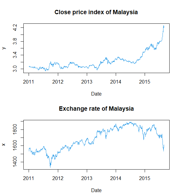
Figure 2 Plots of original signals

Figure 3 illustrates the EMD decomposition of the predictor variable . The decomposed into seven components and one residual component, each decomposition component has distinct physical properties, such as wavelength and frequency.

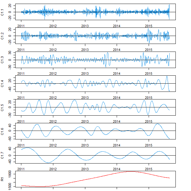
Figure 3 Decomposition of the original signal via EMD

Table 2 illustrates the results of the residual sum of squares error (RSS) values of the EMD-RQR, EMD-LQR and EMD-EnetQR methods at the values of lambda as selected by CV. The results show that the smallest 𝑅𝑆𝑆 value is achieved by the EMD-EnetQR, EMD-LQR yields the second smallest RSS value. RSS values offer an effective approach for selecting and supporting suitable regression models, and the EMD-EnetQR method outperforms previous methods by achieving smaller errors.

Table 2 Performance criteria for real data

	Method		RMSE	MAE	MASE	MAPE	RSS
0.25	EMD-RQR	0.11681787	1.04852	0.60320	6.77596	1.87420	379.2883
	EMD-LQR	0.01168179	1.03828	0.58970	6.62437	1.68978	371.9163
	EMD-EnetQR	0.01460223	1.03831	0.58976	6.62507	1.69144	371.9418
0.50	EMD-RQR	0.18331510	0.95333	0.54764	6.77051	0.93128	313.5484
	EMD-LQR	0.01833151	0.93163	0.53460	6.60931	1.01850	299.4372
	EMD-EnetQR	0.02036834	0.93167	0.53463	6.60959	1.01803	299.5229
0.75	EMD-RQR	0.10003276	0.88387	0.64050	7.96860	3.13043	269.5237
	EMD-LQR	0.02334051	0.87819	0.64413	8.01367	4.05427	266.0702
	EMD-EnetQR	0.02593390	0.87811	0.64359	8.00703	4.01925	266.0214

Figure 4 displays the 10-fold cross-validation estimate plot for EMD-RQR, EMD-LQR and EMD-EnetQR methods with τ values of 0.25, 0.50, and 0.75, respectively. Each plot shows the mean squared error () curve (red dotted line) with error bars indicating one standard error. The y-axis represents , the x-axis represents , and the upper horizontal line indicates the number of nonzero regression coefficients at each log(λ) value.

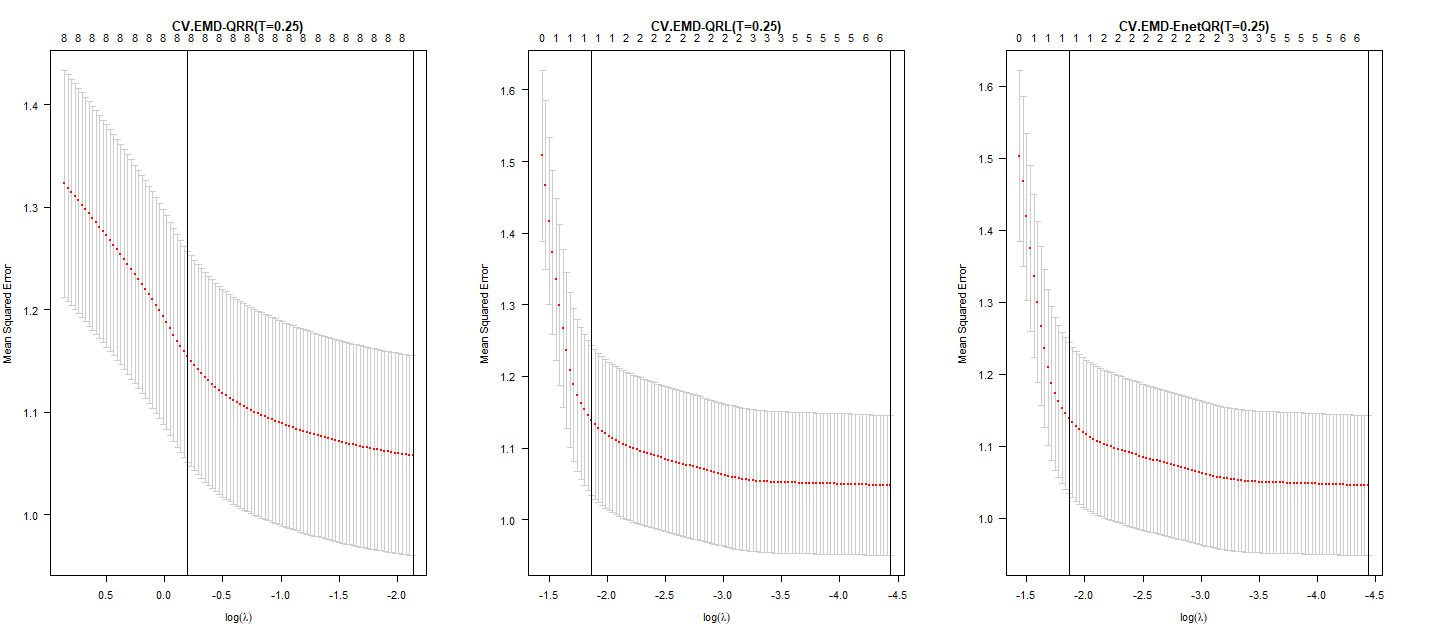
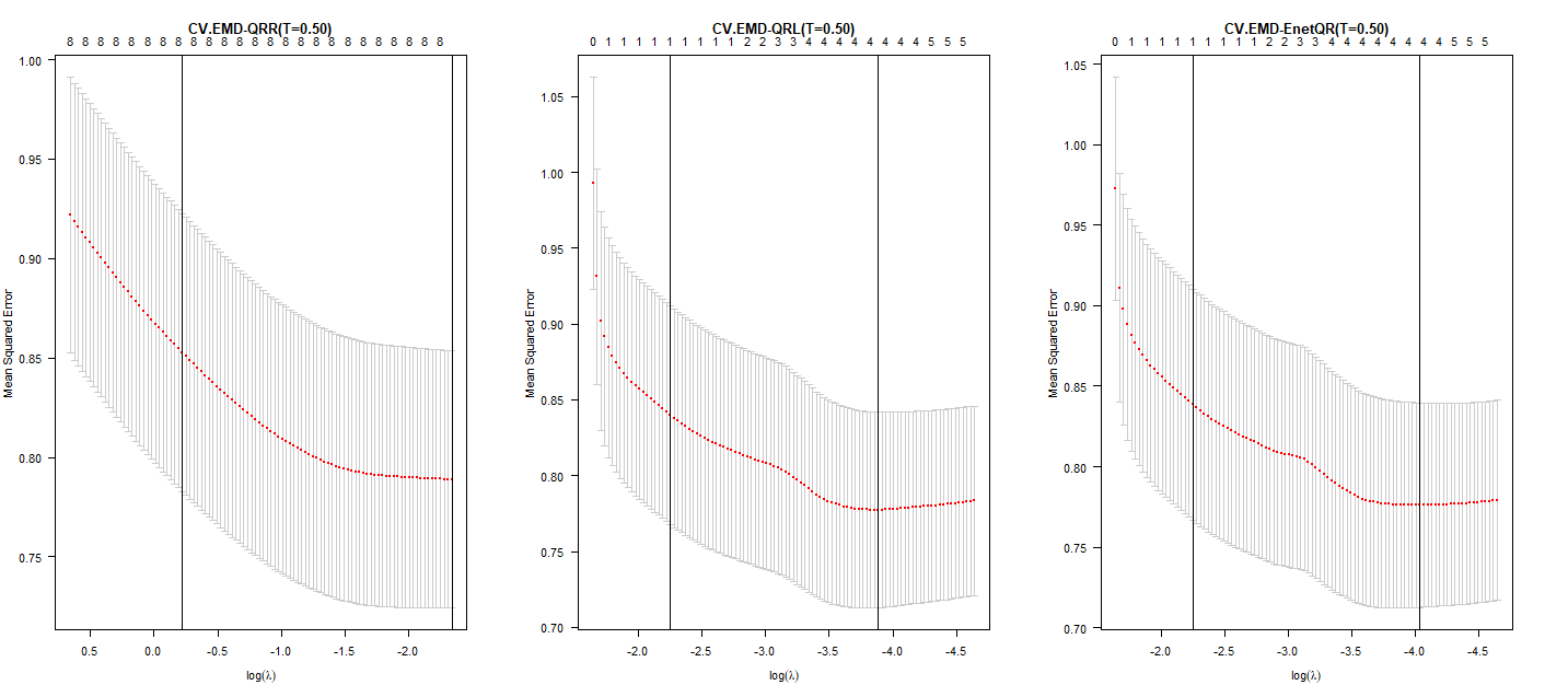
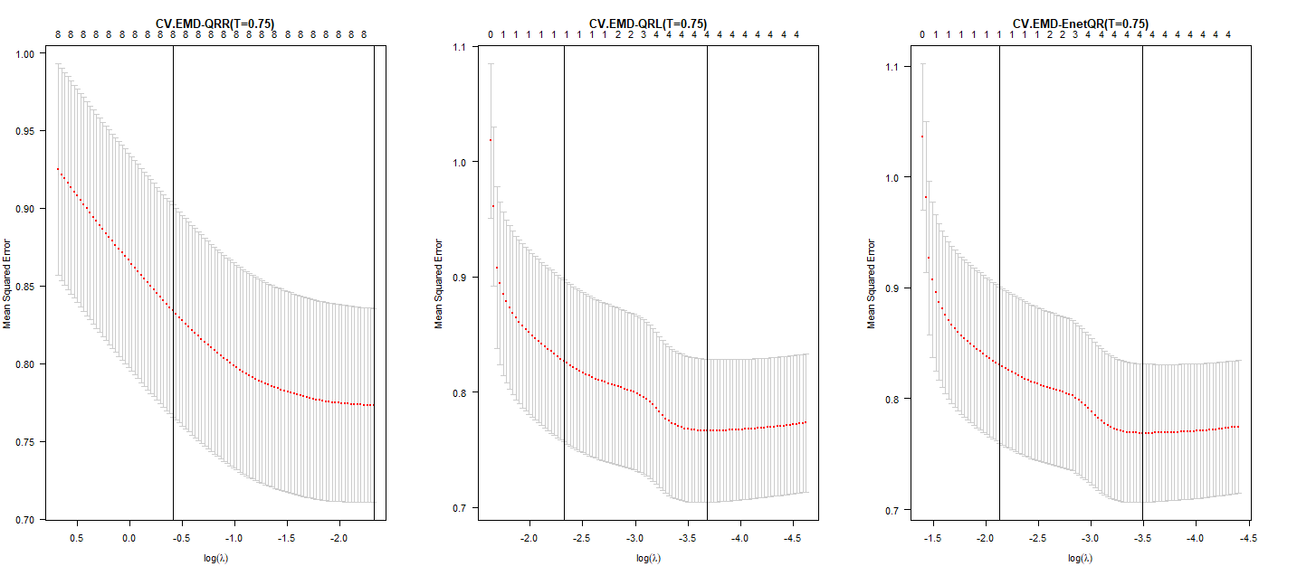Figure 4 10-CV estimation of the tree methods at

The rightmost vertical dotted line indicates the point selected using the minimum MSE rule, while the second line represents the point selected using the minimum plus one standard error () rule. These lines illustrate the number of non-zero regression coefficients selected by each rule. As the Q value increases, the number of non-zero coefficients decrease, thus is selected based on the optimal minimum value.

Table 3 shows the estimation of zero and non-zero coefficients of decomposition components for each of the regression methods used in this study. for example, when τ =0.25 in the EMD-EnetQR method, seven coefficients are selected as non-zero. Whereas in the EMD-LQR method, the number of the coefficients that have been selected equals seven non-zero coefficients, which have the greatest effect on the response variables. The EMD-RQR method selected all the predictor variables in the final model. Thus, this method lost reliability and accuracy for the selection. Therefore, the best method for reducing the number of components and selecting predictor variables with high prediction accuracy is the EMD-EnetQR method.

Table 3 Coefficients estimation for the predictor variables

Variables	Methods
	EMD-QRR			EMD-QRL			EMD-QREnet
	τ =0.25	τ =0.50	τ =0.75	τ =0.25	τ =0.50	τ =0.75	τ =0.25	τ =0.50	τ =0.75
	-0.5431	-0.2815	0.0072	-0.5360	-0.2756	0.0433	-0.5359	-0.2756	0.0416
	-0.0011	-0.0026	0.0014	0	0	0	0	0	0
	-0.0017	-0.0018	-0.0031	-0.0005	0	0	-0.0005	0	0
	-0.0004	0.0007	-0.0019	0	0	0	0	0	0
	-0.0020	-0.0021	-0.0018	-0.0013	-0.0010	0	-0.0013	-0.0010	0
	-0.0021	-0.0014	-0.0036	-0.0005	-0.0003	-0.0048	-0.0006	-0.0003	-0.0047
	-0.0015	-0.0029	-0.0041	-0.0015	-0.0040	-0.0034	-0.0015	-0.0040	-0.0034
	0.0007	-0.0030	-0.0033	0.0012	-0.0028	-0.0038	0.0012	-0.0028	-0.0038
	0.0021	0.0019	0.0026	0.0024	0.0025	0.0033	0.0024	0.0025	0.0033

1. Conclusions

In this study, we compared some of the previously described methods which are EMD-RQR, EMD-LQR and EMD-EnetQR. These methods were used to determine the relationship between the predictor variables and the response variable to enhances model selection accuracy and to address heavy-tailed distributions, heterogeneity, and multicollinearity among the predictor variables. The results of the Simulation Study and real example showed that the EMD-Enet and EMD-LQR methods are considerably more accurate than the EMD-RQR method. Moreover, they are highly capable of identifying the actual predictor variables that have the most significance on the response variable with a reduced prediction error at τ = 0.25, 0.5, and 0.75. In contrast, the EMD-RQR method selected all predictor variables in the final model. The EMD-RQR, EMD-EnetQR, and EMD-LQR methods select the best-fitting model that is free of multicollinearity and heterogeneity. Future research could explore further refinements to these methods or their application in different domains, potentially yielding even more significant insights.

1. References

Akaike, H. (1973). Information theory and an extension of the maximum likelihood principle. Proceedings of the 2nd international symposium on information theory. Second International Symposium on Information Theory, 267–281. https://link.springer.com/chapter/10.1007%2F978-1-4612-1694-0_15

Alhamzawi, R., Yu, K., & Benoit, D. F. (2012). Bayesian adaptive Lasso quantile regression. Statistical Modelling, 12(3), 279–297. https://doi.org/10.1177/1471082X1101200304

Ali, M., Deo, R. C., Maraseni, T., & Downs, N. J. (2019). Improving SPI-derived drought forecasts incorporating synoptic-scale climate indices in multi-phase multivariate empirical mode decomposition model hybridized with simulated annealing and kernel ridge regression algorithms. Journal of Hydrology, 576, 164–184. https://doi.org/10.1016/j.jhydrol.2019.06.032

Al-Jawarneh, A. S., Alsayed, A. R. M., Ayyoub, H. N., Ismail, M. T., Sek, S. K., Ariç, K. H., & Manzi, G. (2024). Enhancing Model Selection by Obtaining Optimal Tuning Parameters in Elastic-Net Quantile Regression, Application to Crude Oil Prices. Journal of Risk and Financial Management, 17(8). https://doi.org/10.3390/jrfm17080323

Al-Jawarneh, A. S., & Ismail, M. T. (2021). Elastic-Net Regression based on Empirical Mode Decomposition for Multivariate Predictors. Pertanika Journal of Science and Technology, 29(1), 199–215. https://doi.org/10.47836/pjst.29.1.11

Alshaybawee, T., Midi, H., & Alhamzawi, R. (2017). Bayesian elastic net single index quantile regression. Journal of Applied Statistics, 44(5), 853–871. https://doi.org/10.1080/02664763.2016.1189515

Ambark, A. S. A., Ismail, M. T., Al-Jawarneh, A. S., & Karim, S. A. A. (2023). Elastic net penalized Quantile Regression Model and Empirical Mode Decomposition for Improving the Accuracy of the Model Selection. IEEE Access, 11(February), 1–1. https://doi.org/10.1109/access.2023.3257032

Ambark, A. S., & Tahir Ismail, M. (2024). PENALIZED QUANTILE REGRESSION AND EMPIRICAL MODE DECOMPOSITION FOR IMPROVING THE ACCURACY OF THE MODEL SELECTION (Vol. 40, Issue 2).

Burgette, L. F., Reiter, J. P., & Miranda, M. L. (2011). Exploratory quantile regression with many covariates: An application to adverse birth outcomes. Epidemiology, 22(6), 859–866. https://doi.org/10.1097/EDE.0b013e31822908b3

Chan, C. T. (1995). Wavelet Basics. In The Journal of the Acoustical Society of America (Vol. 99, Issue 2). https://doi.org/10.1121/1.414569

Classen, T. A. C. M., & Mecklenbrauker, W. F. G. (1980). The Wigner Distribution – a Tool for Time-Frequency Signal Analysis. Part III: Relations with Other Time-Frequency Signal Trasformation. In Philips Journal of Research (Vol. 35, Issues 4–5, pp. 372–389). https://pdfs.semanticscholar.org/442c/69a82eacf4c06a3d534176b516fc4b340857.pdf?_ga=2.23027835.1186082500.1579552434-248343780.1579552434%0Ahttps://pdfs.semanticscholar.org/442c/69a82eacf4c06a3d534176b516fc4b340857.pdf

Davino, Cristina., Furno, Marilena., & Vistocco, Domenico. (2014). Quantile regression : theory and applications. Wiley.

Friedman, J., Hastie, T., & Tibshirani, R. (2010). Regularization Paths for Generalized Linear Models via Coordinate Descent. In JSS Journal of Statistical Software (Vol. 33). http://www.jstatsoft.org/

Hoerl, A. E., & Kennard, R. W. (1970). Ridge Regression: Applications to Nonorthogonal Problems. Technometrics, 12(1), 69–82. https://doi.org/10.1080/00401706.1970.10488635

Huang, N. E. (2005). Introduction to the hilbert-huang transform and its related mathematical problems. In Hilbert-huang Transform And Its Applications (pp. 1–26). https://doi.org/10.1142/9789812703347_0001

Huang, Shen, Z., Long, S. R., Wu, M. C., Snin, H. H., Zheng, Q., Yen, N. C., Tung, C. C., & Liu, H. H. (1998). The empirical mode decomposition and the Hubert spectrum for nonlinear and non-stationary time series analysis. Proceedings of the Royal Society A: Mathematical, Physical and Engineering Sciences, 454(1971), 903–995. https://doi.org/10.1098/rspa.1998.0193

Jaber, A. M., Ismail, M. T., & Altaher, A. M. (2014). Application of empirical mode decomposition with local linear quantile regression in financial time series forecasting. Scientific World Journal, 2014. https://doi.org/10.1155/2014/708918

Khan, D. M., Yaqoob, A., Iqbal, N., Wahid, A., Khalil, U., Khan, M., Rahman, M. A. A., Mustafa, M. S., & Khan, Z. (2019). Variable Selection via SCAD-Penalized Quantile Regression for High-Dimensional Count Data. IEEE Access, 7, 153205–153216. https://doi.org/10.1109/ACCESS.2019.2948278

Koenker, R. (2005). Quantile regression. In Nature Methods (Vol. 16, Issue 6). https://doi.org/10.1038/s41592-019-0406-y

Koenker, R., & Bassett, G. (1978). Regression Quantiles. Econometrica, 46(1), 33. https://doi.org/10.2307/1913643

Li, Y., & Zhu, J. (2008). L1-norm quantile regression. Journal of Computational and Graphical Statistics, 17(1), 163–185. https://doi.org/10.1198/106186008X289155

Masselot, P., Chebana, F., Bélanger, D., St-Hilaire, A., Abdous, B., Gosselin, P., & Ouarda, T. B. M. J. (2018). EMD-regression for modelling multi-scale relationships, and application to weather-related cardiovascular mortality. Science of the Total Environment, 612, 1018–1029. https://doi.org/10.1016/j.scitotenv.2017.08.276

Melkumova, L. E., & Shatskikh, S. Y. (2017). Comparing Ridge and LASSO estimators for data analysis. Procedia Engineering, 201, 746–755. https://doi.org/10.1016/j.proeng.2017.09.615

Sadig, A., & Bager, M. (2018). Ridge Parameter in Quantile Regression Models . An Application in Biostatistics. 8(2), 72–78. https://doi.org/10.5923/j.statistics.20180802.06

Schwarz, G. (2007). Estimating the Dimension of a Model. The Annals of Statistics, 6(2), 461–464. https://doi.org/10.1214/aos/1176344136

Stone, M. (1974). Cross-Validatory Choice and Assessment of Statistical Predictions (With Discussion). Journal of the Royal Statistical Society: Series B (Methodological), 38(1), 102–102. https://doi.org/10.1111/j.2517-6161.1976.tb01573.x

Tibshirani, R. (1996). Regression Shrinkage and Selection Via the Lasso. Journal of the Royal Statistical Society: Series B (Methodological), 58(1), 267–288. https://doi.org/10.1111/j.2517-6161.1996.tb02080.x

Titchmarsh, E. C. (1948). Introduction to the Theory of Fourier Integrals. In Nature (Vol. 141, Issue 3561). https://doi.org/10.1038/141183a0

Xu, Q., Cai, C., Jiang, C., Sun, F., & Huang, X. (2017). Sampling Lasso quantile regression for large-scale data. Communications in Statistics: Simulation and Computation, 47(1), 92–114. https://doi.org/10.1080/03610918.2016.1277750

Yan, A., & Song, F. (2019). Adaptive elastic net-penalized quantile regression for variable selection. Communications in Statistics – Theory and Methods, 48(20), 5106–5120. https://doi.org/10.1080/03610926.2018.1508711

Zaikarina, H., Djuraidah, A., & Wigena, A. H. (2016). Lasso and ridge quantile regression using cross validation to estimate extreme rainfall. Global Journal of Pure and Applied Mathematics, 12(4), 3305–3314.

Zhang, L., Xie, L., Han, Q., Wang, Z., & Huang, C. (2020). Probability density forecasting of wind speed based on quantile regression and kernel density estimation. Energies, 13(22), 1–24. https://doi.org/10.3390/en13226125

Zou, H., & Hastie, T. (2005). Regularization and variable selection via the elastic net. Journal of the Royal Statistical Society. Series B: Statistical Methodology, 67(2), 301–320. https://doi.org/10.1111/j.1467-9868.2005.00503.x