Developing Predictive Models for Time Series Analysis in Stock Markets and Cryptocurrencies

تطوير نماذج تنبؤية لتحليل السلاسل الزمنية في أسواق الأسهم والعملات المشفرة

Sherin M S Tayeh¹, Sefer KURNAZ²

DOI: https://doi.org/10.53796/hnsj64/26

Arabic Scientific Research Identifier: https://arsri.org/10000/64/26

Volume (6) Issue (4). Pages: 511 - 528

Received at: 2025-03-07 | Accepted at: 2025-03-15 | Published at: 2025-04-01

Download PDF

 

---

Introduction

Background of the study

The use of cryptocurrencies has become a widespread phenomenon in the global financial market (Naeem et al., 2023). Cryptocurrencies have provided the rise of new financial assets and thus offer a chance to discover the features of cryptocurrencies. The inclusion of virtual currencies in the worldwide financial markets reached 783 billion U.S. dollars in the year 2013. The significance of the cryptocurrency markets can be tied down to empirical finance, which has increased significantly since then(Carvalho, 2022). Even though the markets of cryptocurrencies are considered rather volatile, their popularity does not seem to drop due to the availability of high returns. One of the famous cryptocurrency assets is bitcoin, which can be used to hedge among a variety of different risks, which include foreign currencies, stock markets, and commodities. The rapid development of digital currencies has brought about the innovation of ambiguous and controversial innovations due to their lack of regulation and high volatility (Sharma Tanmay M Band Snehdeep Raut Aaryan Khanderao, 2023). For this case, there is a need to come up with models and methods relevant to the prediction of prices and cryptocurrency relevant to the scientific community and investors.

Several methodological models can be implemented in the prediction and forecasting of the prices for financial assets, which are determined by the knowledge of the financial analyst. A good example is when the pricing model is considered an appropriate price formation model (Sharma Tanmay M Band Snehdeep Raut Aaryan Khanderao, 2023). The best model to be considered is when given the past dynamics, such as time series analysis and autoregressive models. However, before we embark on this study, we should mention that the forecasting of cryptocurrencies is way different from the forecasting of their financial asset, for example, ordinary fiat currencies. The approach my study tends to investigate is only the time series and coming up with a prediction based on past observations.

1.2. Statement of Problem

Ensuring accurate prediction of the financial time series is an important process since it impacts the decision-making process of key stakeholders such as traders, investors, and financial institutions. Due to the high volatility associated with the financial markets, it is relevant to have precise forecasting models that can be used to provide a competitive edge by enabling the various stakeholders to anticipate market trends and thus strategize on investment strategies. Without accurate predictions, market predictions and overall participation are at risk of a number of uncertainties. Such uncertainties may result in potential financial losses and missed opportunities. Most of the time, poorly informed decisions due to having inaccurate data result in excessive risk exposure, reduced returns, and suboptimal investment choices.

1.3. Research Aim

My research aims to develop a predictive model for time series analysis in the stock market and cryptocurrencies, utilizing advanced machine learning and deep learning techniques to enhance forecasting accuracy.

1.4. Research Objectives

The objectives of my research include:

1. To implement and compare the performance of ARIMA, LSTM, and RNN models in forecasting stock prices and cryptocurrency rates.

2. To explore the integration of external factors into the predictive model to improve their accuracy and adaptation to changing market conditions.

3. To provide insight into financial decision-making among various stakeholders.

1.5. Scope of the Study

The study will operate under the boundaries and focus areas of algorithms and techniques. In this section, the study will focus on the three autoregression integrated moving average (ARIMA), Long Shirt Term Memory (LSTM) networks, and Recurrent Neural Networks. The research will explore the potential of integrating any external factors, for instance, market sentiments and macroeconomic indicators, to enhance the accuracy of forecasting. In addition, the study will evaluate the time series data from the traditional stock markets while focusing on the major stock indices and individual stocks. Major cryptocurrencies, such as Ethereum and Bitcoin, will be evaluated. The data used in this research will be obtained from various online platforms, such as historical data for stocks and cryptocurrencies, as well as the inclusion of external factors such as sentimental analysis data and economic indicators. Furthermore, the study will evaluate the performance of the models based on the metrics used in forecasting the robustness, adaptability, and accuracy of the changing markets. Following this scope will ensure that the study remains focused on the key challenges in financial time series for both the traditional and emerging markets.

2.0. Literature Review

2.1. Introduction to Time Series.

Times series analysis is critical for the adoption and prediction of future outcomes, assessing past performances, and identifying the trends and patterns in various metrics. Because of this, time series analysis offers valuable insights into stock prices, sales figures, and other time-dependent variables (1. Jeris, S. S., Chowdhury, A. N. U. R., Akter, M…. – Google Scholar, n.d.). According to an article from the CFI Team, time series data analysis involves the analysis of the dataset change over some time (Time Series Analysis: Definition, Types & Examples | Sigma, n.d.). Financial analysts can use time series data, such as stock price movement, to analyze a company’s performance. Research by Faster Capital outlines that the time series is a crucial tool for anyone interested in predicting the chaotic movements in markets (Time Series Data Analysis – Definition, Techniques, Types, n.d.). The theory of time series involves the study of data points recorded at specific time intervals. In the financial world, the analysis could mean anything from the stock prices and exchange rates to the interest rates and commodity prices, which will be tracked over weeks, days, months, and even years. The main aim remains to be able to identify goals in the trends, patterns, and correlations that can help predict future movements.

The main core of time series involves statistical methods. Such methods include moving averages, autoregression models, and cointegration tests. Such analysis will help block noise and identify underlying trends. For instance, (SMA) a simple moving average can be implemented to smooth data over a specified prediction period. Often, the financial markets exhibit patterns arising from recurring fluctuations that correspond to a specific period (Time Series Analysis: Chronicles of the Ticker: Time Series Analysis for Financial Data – FasterCapital, n.d.). The identification of such trends can be invaluable for the analysis. For instance, the ‘January effect’ normally observed in the stock market suggests that stocks often increase in January (Derbentsev et al., n.d.). In addition, volatility marketing is strong and inherent in the financial markets and time series analysis, which helps in modeling and forecasting. In this case, we have the ARCH (Autoregressive Conditional Heteroskedasticity) and the GARCH (Generalized Autoregressive Conditional Heteroskedasticity), which are widely used models.

2.2. Machine Learning (ML) and Deep Learning (DL) in Time series

According to Makridakis et al., 2023, it was discovered that the combination of DL models often performs better than a variety of other standard models, both statistical and ML, especially in the case of long-term forecasts and the case of monthly series (Makridakis et al., 2023). ML has always been considered an appropriate tool for time series prediction and forecasting, which is a task that is outlined by the identification of complex patterns. One of the main advantages of ML, when compared to other statistical ones, is that while the statistical methods involve the prescribing of the underlying data generation processes, for instance, in terms of seasonality, they allow for data relationships to be identified and provide an automatic prediction. ML methods make few or no assumptions about the data, and their overall performance relies largely on the adequate availability of data. The model becomes very effective, especially when the predicted series are non-stationary and often display seasonality and trend. Over the years, data availability has stopped being a limiting factor, and thus, more effective algorithms have become available to extract more information from the data. More recently, Deep Learning (DL) has become a promising alternative to standard forecasting.

According to Makridakis et al., 2023 as a result of various studies comparing the accuracy provided by ML and statistical methods, we later found that through the M4 commentators, recent advances in DL have proven that the concept has not been evaluated to its full potential (Makridakis et al., 2023). However, today, the situation has changed since powerful DL packages have been available online to process time series forecasting. Previous researchers have developed models for forecasting market trends. According to Summit (2021), the DeepAR signifies an RNN-based probabilistic forecasting model that was proposed by the Amazon Company (Specialized Deep Learning Architectures for Time Series Forecasting – Sumit’s Diary, n.d.). The model is relevant for training from large numbers related to time series. The model operated by learning seasonal behavior and the dependencies without relying on manual engineering. In addition, the system is able to incorporate cold items with the use of limited historical data. Assuming t0 is the forecast creation time (i.e., the step in which the forecast of the future horizon must be generated, we will aim to model the following conditional distribution)

P(z_i,t_0:T| z_i,1: t₀-1,X_i, 1:T):

t_0:T represents the future horizon

1: t₀-1 represents the historical lag

X_i, 1:T represents the covariates.

While implementing the autoregressive recurrent for the network, we will further represent the model of distribution as the product of likelihood factors.

z_i,1: t₀-1 will represent the autoregression

RNN Output

is the model parameters

2.3. ARIMA, LSTM, and RNN Models

2.3.1. ARIMA Model

According to the article from Caroprese (2024), ARIMA (Autoregressive Intergrated Moving Average) is a prominent method for time series analysis that offers a classical statistical approach. The models tend to understand a time series internal structure through the examination patterns in the data sequence(Caroprese et al., 2024). It operates on the axioms of three components: autoregression, moving average, and integration. ARIMA models hold significance in the prediction of stationary time series data without seasonality and trends. This implies that the statistical properties, such as mean and variance, stay constant over time. The key benefits outlined by the model include;

Ability to work well with stationary and linear data

It is simple to implement

Offers fast training compared to the other complex model

Offers interpretable insights into the data patterns

However, the ARIMA model normally struggles when it comes to the implementation of nonlinear patterns or multiple seasonality. It is in such instances that more advanced machine learning models, such as Long Short-Term Memory (LSTM) networks, always excel.

Researchers Caroprese et al. (2024) outlined ARIMA as the combination of both AR (Autoregression) and MA (Moving averages) processes(Caroprese et al., 2024), which constitutes the overall model used in the time series. The simple model of the AR model can be illustrated in a linear process by the equation.

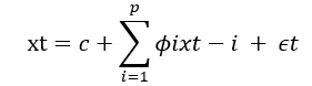
tx represents the stationary variable

c is the constant

are the autocorrelation coefficients at lags 1,2,…,p and

2.3.2. LSTM Model

According to the article from Caroprese (2024), LSTM signifies the set of recurrent networks ideal for the modeling of long-term dependencies in the time series(Caroprese et al., n.d.). The model offers benefits such as :

• Ability to capture non-linear relationships

• Automatic learning of multiple seasonality

• Achievement of greater accuracy for complex data

• Require access to more data and computing resources.

According to Siami-Namini et al. (2019), The LSTM is capable of remembering the values from earlier stages for the overall purpose of future interpretation(Siami-Namini et al., 2019). Before we delve into and consider the makeup of an LSTM, we need to have an acute knowledge of ANN (Artificial Neural Network) and RNN (Recurrent Neural Network). The LSTM is a special kind of RNN that essentially features the memorization of earlier trends of sequence data. This is made possible through some examples of gates and memory lines, which are incorporated into the LSTM. Each of the LSTMs represents a set of system modules and cells where the data streams will be stored and captured. The cell holds a representation of a specific transport line that connects out of another module, one used in conveying from the past and gathering them for the present cell. Resulting of the use of cell technology, data in every cell is at risk of being exposed, added, and filtered for the next cell. For this reason, the gates, which are based on the sigmoidal neural network layer, enable the cells to selectively let data pass through. Every sigmoidal layer comprises a number in the range of zero to one, outlining the amount of every segment of data having to be sorted in each cell. For example, the number zero means let nothing pass through, whereas one signifies let everything pass through.

2.3.3. RNN Models

According to the AWS website, it is a model trained to convert any sequential data input into a specified sequential output(What Is RNN? – Recurrent Neural Networks Explained – AWS, n.d.). Sequential data input includes time-series data in the case where sequential components interrelate based on complex syntax and semantic rules. An article from the IBM website illustrated how an RNN works similarly to a feedforward and conventional neural network (CNN). They similarly utilize training data to learn (What Is a Recurrent Neural Network (RNN)? | IBM, n.d.). One distinguishing factor among RNNs is their ability to take memory as they take information from the inputs prior and use it to influence the current inputs and outputs (Fear and Greed Index – Investor Sentiment | CNN, n.d.). This is contrary to the case of traditional inputs, which assume that inputs and outputs are independent of one another.

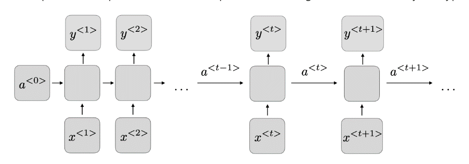
Figure 1: Architecture of a Recurrent Neural Network.

According to the Standford website, Figure 1 above, for every timestep t, the activation a^<t> and the output y^<t>is an expression equation as follows(CS 230 – Recurrent Neural Networks Cheatsheet, n.d.).

a^<t> = g₁(W_aa a^<t-1> + W_axx^<t> + b_a) and y^<t> = g₂(W_ay a^<t> + b_a)

W_aa, Wax, ba_{, Way, and a} stand for the coefficients that are shared temporarily, and g₁ and g₂ represent activation functions.

RNN comes with several benefits, such as;

• The broad possibility of processing inputs of any length

• The model size does not increase with the size of the input

• Computational task account for historical information

• The weights are shared across time

The disadvantages of the RNN include:

• The overall computational is slow

• There is difficulty in accessing information dating from way back

• The model cannot consider any future inputs for the current state

2.4. External Factors in Forecasting

External factors such as macroeconomic indicators and market sentiments have brought about a significant change to the predictive models for time series analysis in the financial markets. The factors offer additional information that enhances the predictive accuracy of models such as LSTM, ARIMA, and RNN. According to El-Azab (2024), the ability to accurately predict market movements has been a long-standing challenge in finance. With the dominance of traditional models based on economic indicators and historical price data, we have limited, if not minimal, predictive power, especially when it comes to the face of emotional and psychologically driven dynamics as characterized in the financial markets(El-Azab et al., n.d.). Through monitoring and quantifying sentimental expressions from online discussions, news articles, and social media, we can incorporate real-time measures to assess market psychology and investor sentiments. Such sentimental data is relevant in identifying emerging trends, differentiating different temporary market fluctuations from long-term shifts, and identifying emerging trends.

Market sentiments outline the overall attitude of the investors towards a particular market or asset. The assets are normally captured through news articles and social media posts, among other channels. According to CNN (2024), sentimental analysis makes use of natural language processing (NLP) techniques to quantify this sentiment into numeric values(Fear and Greed Index – Investor Sentiment | CNN, n.d.). When such external factors are combined with the traditional ARIMA model through various extensions such as ARIMAX, we can improve ARIMA’s short-term forecasting ability. In the case of LSTM and RNN, macroeconomic indicators are treated as additional features for the input alongside historical data prices. Such models can capture complex temporal dependencies between macroeconomic conditions and market behavior. Furthermore, deep learning models like LSTM and RNN are inherent and capable of understanding multiple input features, including sentimental data. Previous researchers have included sentimental scores along with price data, which enable the model to learn complex relationships between the sentiment and the market.

According to Sarika (2023), the performance of various stock markets can be directly attributed to a broader financial marketplace. Macroeconomic indicators include interest rates, inflation, GDP growth, and unemployment rates(Keswani et al., 2024). In an analysis of the comparison between macroeconomic factors and Indian stock prices, the researcher managed to deduce a negative correlation between government policies, interest rates, and inflation. On the other hand, the researcher was able to conclude that there was a positive correlation between disposable income, GDP, and Foreign Institutional Investors. In addition, theoretic and empirical work from researchers such as Chen et al. (1986) has shown that fluctuations in macroeconomic variables are capable of impacting future trends in dividend rates, stock prices, and discount rates(Chen et al., n.d.). Let us have an instance where the disposable income of a household has increased; the household will have an option of either spending or saving, both having a selective impact on the economy. In such a situation, the surge in consumption will also trigger an upswing in corporate sales and earnings, thus enhancing the value of individual stock companies.

3.0. Methodology

In this section, we will follow a step-by-step procedure relevant to the development of a predictive model for stock market and cryptocurrency price forecasting. The methodology will integrate traditional statistical models (ARIMA) and deep learning techniques (RNN and LSTM) to compare the effectiveness of the time series dynamics (Van Houdt et al., 2020). The dataset was obtained from the Kaggle website, which is an online published website that allows its users to be able to locate and collaborate on published databases and use GPU-integrated notebooks

3.1. Data Collection

An appropriate dataset was selected from Kaggle. Kaggle is one of the most trusted sites for obtaining stock historical data and cryptocurrency prices (Cryptocurrency Historical Prices, n.d.). The good is that the datasets have been verified and are open-sourced for public research and scrutiny. Below is a table description of the features of my datasets.

Feature	Description	Unit
Timestamp	Represents the date and time of the recorded data point, typically in UTC format.	DateTime (UTC)
Open Price	Represents the price of Bitcoin at the beginning of the interval.	Million USD
High Price	Represents the highest price of the Bitcoin during the time interval.	Million USD
Low Price	Represents the lowest price of the Bitcoin during the time interval.	Million USD
Close Price	Represents the price of the Bitcoin during the end of the time interval.	Million USD
Volume of BTC	Represents the total number of Bitcoins traded during the time interval.	Million USD
Volume of Currency	Represents the trading volume in fiat currency during the time interval.	Million USD
Weighted Price	This is the average price of the Bitcoin during the interval, weighted by volume.	Million USD

Table 1: Description of the Dataset Feature(Iqbal et al., 2021.)

Figure 1 below represents the explanatory analysis of each feature according to the time series from which the data has been collected.

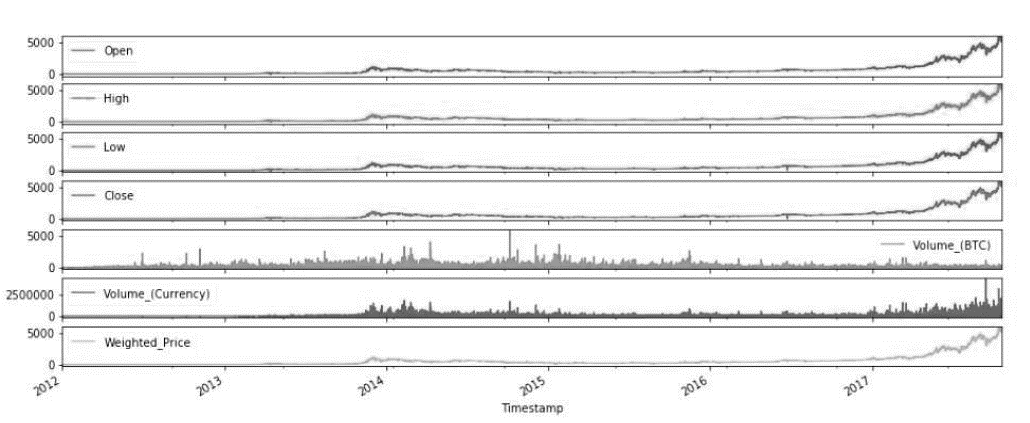
Figure 2: Explanatory Analysis of Every Feature of the Dataset(Iqbal et al., 2021.)

3.2. Data Preprocessing

In order to prepare the dataset for modeling, several steps were conducted. Yes, the data set from Kaggle might be clean; however, we may never be certain. To ensure the dataset was prepped for the time series forecasting, first, all the rows containing the missing or null values were removed to prevent any potential bias during the model training. For simplicity and concentration on trend prediction, only the ‘Close’ price features were selected as the target variable for forecasting. Since the Recurrent Neural Network (RNN) and Long-Short Term Memory (LSTM) models are sensitive to input scale, the outlined features were normalized using the MinMaxScaler, relevant for transforming the data into a range between 0 and 1(Iqbal et al., 2021.). Eventually, the dataset was divided into training the data and testing sets with an 80:20 ratio, thus ensuring the chronological order of the data was maintained, preventing data leakages, and preserving the temporal structure essential for the time series modeling.

3.3. Model Development

3.3.1. ARIMA Model

The ARIMA model was implemented using the statsmodels library. To configure our parameters, the p(autoregressive order), d(degree of differencing ), and q (moving average order) were initially conditional by analyzing the Autocorrelation Function (ACF) and the Partial Autocorrelation Function(PACF) plots. Such parameters were later fine-tuned through a grid search and let to identify the optimal combination that minimized forecasting error. After the model had been trained on the historical data, it was later used to make predictions for test periods. The performance of the ARIMA model was assessed using common evaluation metrics, including the Mean Squared Error (MSE), Root Mean Squared Error (RMSE), and the coefficient of determination (R2 score), thus providing insights into the model’s accuracy and predictive capability.

3.3.2. Recurrent Neural Network (RNN

The Recurrent Neural Network (RNN) model was developed using the Tensor Flow /Keras framework to capture the temporal dependencies in the Bitcoin price data. The architecture will include two Simple RNN layers to process sequential input, followed by a Dense output layer to generate the predicted closing price(Yazdan et al., n.d.). A sliding window approach will be employed to prepare the input for the model; here, the sequences of consecutive time steps were used to predict the next day’s closing price. Such a method allowed the be able to learn from the recent patterns and trends in the data. The RNN model was trained on the normalized dataset, leveraging its inherent capability to model sequential data effectively.

3.3.3. Long Short-Term Memory (LSTM)

The Long Short-Term Memory (LSTM) was implemented to improve forecasting accuracy by capturing both short -and long-term temporal dependencies in the time series data. The architecture comprised one LSTM layer integrated with dropout regularization to prevent overfitting, followed by a Dense layer for output generation. In a similar manner to the RNN setup, input sequences were structured using a sliding window approach where every sequence of time steps was implemented to predict the succeeding day’s closing price. LSTM was chosen over the standard RNNs due to its essential capability to overcome the vanishing gradient problem over standard RNNs due to its inherent ability to overcome the vanishing gradient problem through its gated cell architecture. Which enables it to retain information over long time intervals. This makes LSTM an effective approach for financial time series forecasting, where both recent fluctuations and broader trends can influence future values (Van Houdt et al., 2020).

3.4. Model Training

For this section, we implemented both the training of RNN and LSTM for the purposes of producing optimal learning while ensuring a minimum overfitting. The models were trained with a batch size of 50 to 100 epochs with a batch size of 32, hence balancing training efficiency and stability. The Mean Squared Error (MSE) was implemented as the loss function to quantify the prediction error, as it is well suited for regression tasks involving continuous values (Hodson et al., 2021). For adaptive learning rate and efficient convergence properties, the Adam optimizer was implemented. To further enhance model generalization, early stopping was implemented, validation loss was monitored, and training was halted if no improvement was observed over successive epochs. In addition, model checkpoints were used to save best-performing weights based on validation performance, hence ensuring the final model used for prediction did not overfit the training data.

3.5. Model Evaluation

For the assessment of the performance and the forecasting model, a unique combination of the qualitative metrics and the quantitative visualization metrics techniques were employed. The main evaluation metrics included Mean Squared Error (MSE), Root Mean Squared Error (RMSE), and the R2 score (coefficient of determination). The MSE measured the average of the squared differences between the actual and the predicted values, thus emphasizing larger errors and serving as a key indicator of model accuracy. RMSE, the square root of the MSE, provided an interpretable error value in the exact units as the original data, making it easier to comprehend in practical terms. The R2 was relevant for the evaluation of how well the model captured the variability of the target variables, with values closer to 1 indicating better predictive performance. Outside numerical figures and metrics, visual comparisons were made by plotting actual versus predictable closing prices over the test period. Such plots allowed for qualitative evaluations of the model’s trend-tracking capabilities and helped identify any systematic deviations or lags in the predictions.

3.6. Tools and Technologies Used

The implementation of the experiment in this study was carried out using Python 3.11, which is a widely adopted programming language in the data science and machine learning community. The language offers good and proper readability, an extensive ecosystem, and library flexibility. Visual Studio Code served as the primary integrated development environment (IDE) chosen because it offers lightweight design, robust support, and rich extension features, including features such as IntelliSense, debugging and Git Integration, and Jupiter Notebook support. The core data processing and numerical operations included Pandas and NumPy, which offer effective handling of large datasets and powerful data manipulation capabilities (McKinney, 2022). For Machine learning preprocessing, evaluation, and utility functions, Scikit-learn was employed. Deep learning models such as RNN and LSTM were implemented using TensorFlow and Keras, which provided scalable model training and easy-to-use APIs for building complex neural network architecture (Nguyen et al., 2025). Various time series forecasting using the ARIMA model was achieved with the States model’s library, which supports a wide range of statistical and econometric tools. Data visualization was facilitated by Matplotlib and Seaborn, both of which allowed the creation of detailed plots and visual insights into model performance and data trends.

3.7. Workflow Summary

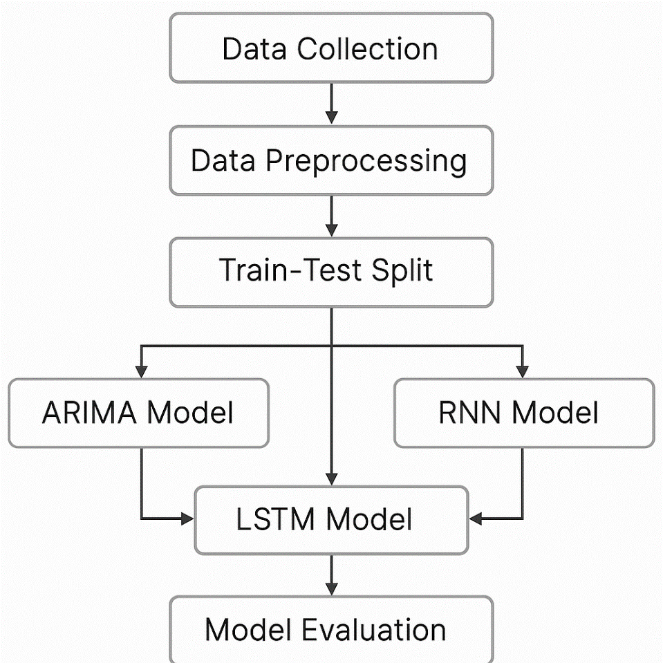
Figure 3: Illustration of the Workflow Summary

The project workflow will begin with the data collection from Kaggle, which is then preprocessed for quality and consistency. The data will hence be used to develop a machine learning model (ARIMA, LSTM, and RNN), which is suitable for the time series analysis of our stock market and cryptocurrency trends. Every model will undergo training and testing using a portion of the dataset, having the performances evaluated using metrics such as the RMSE and MAE. Comparative analysis will thus help determine the most accurate model. The final step involves visualization of the predictions to interpret the results and draw insights for practical application for financial forecasting.

4.0. Results and Discussion

4.1. Introduction

The chapter will outline the results driven by the application of the selected predictive models on the stock market and current crypto datasets(Cryptocurrency Historical Prices, n.d.). The models were evaluated based on their accuracy, prediction error, and sustainability for financial series data. The outcomes of the analysis are discussed below, with supporting visualization and performance metrics to illustrate the strengths and limitations of every method. The historical Bitcoin market data specifically focused on the closing price trend from 2013 to 2021. The primary goal was to observe significant trends, periods of high volatility, and anomalies that could inform the prediction modeling in subsequent chapters.

4.2. Model Evaluation Metrics

For the evaluation of the performance of the forecasting models, three standard evaluations were carried out, namely: Root Mean Square Error (RMSE), Mean Absolute Error (MAE), and the R-squared (R2) score. The RMSE quantifies the average magnitude of the prediction errors, giving higher weight to the larger errors. The MAE measures the average of the absolute differences between the predicted and the actual values, providing a more interpretable error magnitude. The R2 score indicates how well the model explains the variance in the actual data, with a score closer to 1 representing a better fit. The metrics obtained were consistently applied across all three models to ensure a fair and objective comparison of their predictive capabilities. The evaluation results for each model were compiled based on their predictive capabilities, and thus, their evaluation results for every model were compiled into the comparative table, which can be integrated directly into Jupyter Notebook for transparency and reproducibility.

4.3. ARIMA Model Results

The ARIMA Model was trained with the cryptocurrency dataset. The ARIMA model was implemented to predict and analyze the closing prices of Bitcoin over time, thus utilizing the cryptocurrency data. The model was trained on the closing price series extracted from a cleaned and time-indexed dataset. Even though ARIMA is a robust linear time series forecasting method, its performance revealed significant limitations. Bitcoin is inherently volatile, and non-linear behaviors posed challenges for the ARIMA linear assumption. Thus, it resulted in the model struggling to capture the complex dynamic and rapid price swings characteristics of the crypto market. The evaluation results showed significant differences between the actual and predicted values through Root Mean Square Error (RMSE) of 29,635.32 and Mean Absolute Error (MAE) of 28,853.26. The R-squared (R²) score of -5.88 indicates inferior performance compared to a basic mean predictor since the model explained no data variance. The negative R² score demonstrates that ARIMA experienced failure in modeling the extreme price fluctuations together with non-linear Bitcoin price trends.

4.4. LSTM Model Results

The LSTM Model was implemented to address the limitations of traditional linear models like ARIMA, particularly in modeling the highly volatile and non-linear nature of cryptocurrency price movements. An LSTM network analyzed Bitcoin closing prices through its structure that detects temporal sequences and patterns within time-based information. The analysis data underwent MinMaxScaler normalization, while the sequences allowed the model to understand temporal patterns more effectively. The LSTM architecture contained stacked layers with 50 units between each layer before using the dense output layer to extract complex time series features. The 20-epoch training period proved the model suitable for fitting data while preventing overfitting because it managed sequences of specific lengths and had small batch sizes. Evaluation measurements confirmed that the Root Mean Square Error (RMSE) reached 1,618.47 while the Mean Absolute Error (MAE) achieved 1,297.02 with improved results when compared to ARIMA. The R-squared (R²) score of -4.59 indicates a minimal increase in understanding volatility across extremely volatile cryptocurrency data despite its unfavorable value. Such results proved the LSTMS potential as a more robust model for financial time series forecasting, especially in dynamic markets like cryptocurrencies.

4.5. RNN Model Results

The RNN model was employed to evaluate the effectiveness of the traditional sequence-learning architectures in forecasting cryptocurrency prices. The RNN had a simpler design than LSTM because it consisted of two stacked SimpleRNN layers with a dense output layer attached. The training occurred using the Bitcoin closing price dataset after normalization and sequence-based time-step preparation for dependency learning. Despite the RNN’s inherent capacity to handle sequence data, it lacks the memory gates of LSTM, making it more vulnerable to vanishing gradients. The assessment of the RNN model revealed its performance restrictions. The evaluation of the RNN model produced an RMSE of 2,763.57 while its MAE reached 2,437.23, which showed improved forecast precision compared to ARIMA, yet it performed worse than the LSTM model. The obtained R-squared (R²) score was -15.30, which indicates a very poor model fit because the model failed to adequately explain the data variance.

4.6. Comparative Analysis

The summary of the three models was compared since each model provided data with significant disparities. The ARIMA model produced the most inaccurate results when measured by RMSE 29,635.32 and MAE 28,853.26. The results indicate that ARIMA fails to produce reliable predictions within cryptocurrency markets that display high volatility and non-linear features. The LSTM model outperformed other models by producing both a minimum RMSE of 1,618.47 and an MAE of 1,297.02 because it excels at detecting complicated time-based sequences along with sudden market shifts. The RNN model performed better in trend prediction than ARIMA but failed to match LSTM performance because it yielded an RMSE of 2,763.57 and an MAE of 2,437.23 during the prediction assessment period.

The R² scores of all three predictive models generated negative results, establishing them as inferior to a simple mean outcome predictor. ARIMA produced a negative R² value of -5.88 compared to RNN’s worse performance of -15.30, which demonstrates a significant deviation from market reality. Despite negative R² scores, LSTM demonstrated a better capability to discover meaningful patterns in the data, which resulted in its R² score of -4.59. LSTM stands out as the most effective model for cryptocurrency time series forecasting among these three because it achieved better performance despite generating negative R² values.

Model	Dataset Type	RMSE	MAE	R2 Score
ARIMA	Crypto	29635.32	28853.26	-5.88
LSTM	Crypto	1618.47	1297.02	-4.59
RNN	Crypto	2763.57	2437.23	-15.30

Table 2: Comparative table analysis of the three models

Out of the three models analyzed for cryptocurrency forecasting, the ARIMA model struggled the most; the RNN improved significantly; however, LSTM was the best choice among the three, this was due to its ability to model non-linear dependencies and long-term trends effectively

4.7. Visualization of Results

The line plot depicts two predictive accuracy metrics through which both ARIMA and LSTM and RNN models can be evaluated using Root Mean Squared Error (RMSE) and Mean Absolute Error (MAE). Three forecasting models, namely ARIMA, LSTM, and RNN, are represented on the x-axis, whereas error values are shown on the y-axis. The graph contains two separate lines that represent RMSE as well as MAE values. Performance metrics reveal that ARIMA produced the highest error levels as both RMSE and MAE exceeded the values of RNN, and finally, LSTM demonstrated the lowest errors for both aspects. Visual evidence indicates that the LSTM model achieves better accuracy and stability in forecasting cryptocurrency price movements because its results show a steady downward pattern compared to ARIMA.

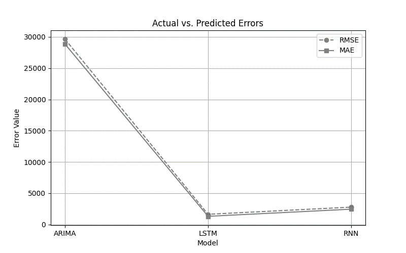
Figure 4: Illustration of the RMSE & MAE variations across models

The bar chart presents the residuals calculated from actual and predicted values for ARIMA alongside LSTM and RNN models. The bar chart displays three models on the x-axis and shows residual magnitudes through bar heights on the y-axis. The average absolute residual errors for every model type appear as individual bar segments. ARIMA exhibits the most significant residuals, which indicate a large number of prediction errors. The RNN model produces error residuals, which are at an intermediate range, thus demonstrating somewhat advanced error management capabilities. LSTM provides the most effective error reduction through its short residual length. LSTM produces forecast results that demonstrate superior accuracy while maintaining smaller deviations when compared to actual values according to the bar chart presentation.

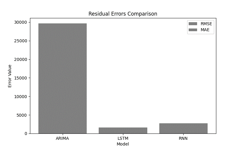
Figure 5: Model Residuals (Prediction Errors)

The graphical display compares the three models across the x-axis and shows the R² score measures on the y-axis. A reference line located at R² = 0 serves to show the performance level of a basic prediction model that uses the mean value for guessing. The R² values of all three models exist below the baseline reference line at zero, which indicates that each model performed worse than mean-based predictions. The RNN model makes the most pronounced deviation below the zero baseline, indicating it struggles to capture data variations, yet LSTM achieves the nearest proximity to zero, indicating a superior model fit.

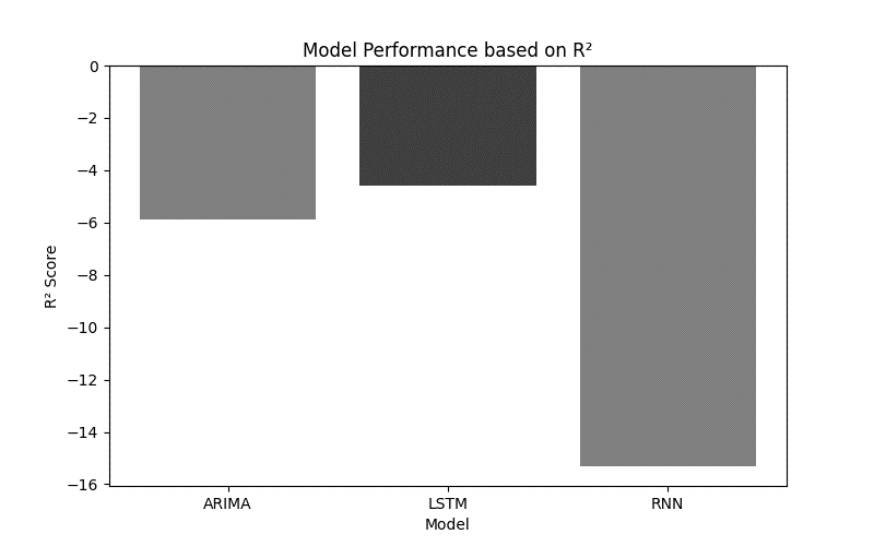
Figure 6: Trend Visualization – R² Score Comparison

4.8. Results Interpretation.

The results show that among these analysis models, the LSTM shows the best accuracy through its minimal RMSE and MAE values. The ability of LSTM to master long-term dependencies and analyze non-linear data patterns from financial time series data is the main reason behind its superior performance. ARIMA and RNN models prove less suitable than LSTM models since they produce substantially higher error metrics when analyzing cryptocurrency market price changes. In addition, the negative R² scores from all models exhibit difficulties in predicting volatile data because simple mean-based projections perform better than any model in this case. The R² score obtained by LSTM stands out as the most positive, which strengthens its superiority in generating dependable forecasts.

4.9. Summary of the Results

The findings assessed predictive model performance on cryptocurrency price data through three predictive models, which used RMSE, MAE, and R² as their evaluation metrics. The LSTM model surpassed the remaining models by producing the lowest prediction errors of RMSE 1618.47 while also delivering MAE 1297.02, which indicates its superiority in predicting market movements. The high errors from ARIMA stood out because the model registered an RMSE value of 29635.32, together with an MAE value of 28853.26, as it struggles with non-linear data that contains high variance. The RNN demonstrated better performance than ARIMA yet fell substantially short compared to LSTM. The calculated R² scores were negative for every experimental model; therefore, a simple mean prediction delivered better results compared to each formal model fit. The results validate LSTM as the model that excelled at identifying complex patterns because it demonstrated the lowest negative R² value (-4.59).

5.0. Discussion

According to the first objective, LSTM produced better forecasts than both ARIMA and RNN models because it generated the most accurate values of RMSE and MAE, which proves its superiority at identifying complex temporal relationships in time series data. The research verifies that deep learning algorithms, particularly LSTM, provide better results with volatile financial data due to their ability to meet the requirement for identifying suitable forecasting methods.

In relation to the second and third objectives, the study offers a strong foundation for the cooperation of external variables, such as economic indicators, social media sentiments, and trading volume iterations. The study delivers essential insights that financial analysts, along with traders and institutional investors, need to make data-based decisions. This research defines LSTM as the most promising model while advancing the capability for informed risk assessment strategic planning, as well as resilient financial forecasting in stock and crypto domains.

Conclusion

In conclusion, the deeply volatile non-linear crypto market behavior demanded the identification of a system that would excel at identifying intricate temporal patterns. A sequential methodology enabled the researchers to perform preprocessing steps on the data, including normalization, in addition to handling missing values and selecting relevant features before applying standard performance metrics for model evaluation (RMSE, MAE, R²). The experimental framework involved Python 3.x with VS Code, and it incorporated NumPy, Pandas, Scikit-learn, TensorFlow/Keras, and Statsmodels data science libraries.

The proposed model achieved the best forecasting capability by producing 1,618.47 as its RMSE value alongside 1,297.02 for MAE, which established its status as the most dependable model. The negative R² value of -4.59 displayed in the experiment did not hinder the model’s superiority to both RNN and ARIMA throughout all test periods. The RNN model demonstrated a slightly better performance than ARIMA with an RMSE result of 2,763.57 along with MAE of 2,437.23 and R² value at -15.30, but it failed to effectively handle long-range dependencies because of its limited structural depth.

References

1. Amazon: What is RNN? https://aws.amazon.com/what-is/recurrent-neural-network/#:~:text=A%20recurrent%20neural%20network%20(RNN,complex%20semantics%20and%20syntax%20rules.
2. Amidi, A., & Amidi, S. (2018). Vip cheatsheet: Recurrent neural networks. https://stanford.edu/~shervine/teaching/cs-230/cheatsheet-recurrent-neural-networks
3. Caroprese, L., Pierantozzi, M., Lops, C., & Montelpare, S. (2024). DL2F: A Deep Learning model for the Local Forecasting of renewable sources. Computers & Industrial Engineering, 187, 109785. https://www.sciencedirect.com/science/article/pii/S0360835223008094#:~:text=In%20essence%2C%20DL%20F%20is,Recurrent%20Unit%20(GRU)%20type.
4. Carvalho, M. F. (2022). Explosive Behaviour in Cryptocurrency Prices (Master’s thesis, Universidade Catolica Portuguesa (Portugal)). https://www.proquest.com/openview/f2fb841fffe08dd19d094be0d2e97295/1?cbl=2026366&diss=y&pq-origsite=gscholar
5. CFI Team (Time Series Data Analysis): https://corporatefinanceinstitute.com/resources/data-science/time-series-data-analysis/
6. Chen, N. F., Roll, R., & Ross, S. A. (1986). Economic forces and the stock market. Journal of Business, 59, 383–403. https://www.jstor.org/stable/2352710
7. CNN Business : Fear & Greed Index (2024) https://edition.cnn.com/markets/fear-and-greed
8. Cole Stryler (2024) IBM: What is a recurrent neural network (RNN)? https://www.ibm.com/topics/recurrent-neural-networks
9. Derbentsev, V., Datsenko, N., Stepanenko, O., & Bezkorovainyi, V. (2019). Forecasting cryptocurrency prices time series using a machine learning approach. In SHS Web of Conferences (Vol. 65, p. 02001). EDP Sciences. https://www.researchgate.net/publication/333464180_Forecasting_cryptocurrency_prices_time_series_using_machine_learning_approach
10. El-Azab, H. A. I., Swief, R. A., El-Amary, N. H., & Temraz, H. K. (2024). Machine and deep learning approaches for forecasting electricity price and energy load assessment on real datasets. Ain Shams Engineering Journal, 15(4), 102613. https://www.sciencedirect.com/science/article/pii/S2090447923005026
11. Faster Capital (2025) Time Series Analysis: Chronicles of the Ticker: Time Series Analysis for Financial Data: https://fastercapital.com/content/Time-Series-Analysis–Chronicles-of-the-Ticker–Time-Series-Analysis-for-Financial-Data.html
12. Hodson, T. O., Over, T. M., & Foks, S. S. (2021). Mean squared error, deconstructed. Journal of Advances in Modeling Earth Systems, 13(12), e2021MS002681. https://agupubs.onlinelibrary.wiley.com/doi/full/10.1029/2021MS002681
13. Iqbal, M., Iqbal, M. S., Jaskani, F. H., Iqbal, K., & Hassan, A. (2021). Time-Series Prediction of Cryptocurrency Market using Machine Learning Techniques. EAI Endorsed Transactions on Creative Technologies, 8(28). https://d1wqtxts1xzle7.cloudfront.net/79664921/eai.7-7-2021-libre.pdf?1643303268=&response-content-disposition=inline%3B+filename%3DTime_Series_Prediction_of_Cryptocurrency.pdf&Expires=1746126994&Signature=e8FxA-fKzPHuABRP5CEKzWPfvdUQPwFZJZGuVryVfrPhYYx3IxHMPsCkCmvnzAbDHCrlnZidRjrzllDyykpv2vbLBUIHN-TsE1CXAYyoQfuaekUkF4qYniCDf~ZZxK2rLcOQoPdW-WY~CtkXiMu04xpzC6Jrlhvryz-Is1b9Wx66wBYH0sA2Qr1M9bcGZfz5vL040UZOtb~2VD7Q8WHYTHrf4t2n27N0xYxJ0ZqW0l~a22dOrR~gjNEBHMFCrbe0zCKCExtjBz5msSjUoejUTmHC0~ACPTMWbzVFgmbliYnM4GrviwNOfusj9doy8p1ric-xNwybxz0QLLGovA5kAw__&Key-Pair-Id=APKAJLOHF5GGSLRBV4ZA
14. Jeris, S. S., Chowdhury, A. N. U. R., Akter, M. T., Frances, S., & Roy, M. H. (2022). Cryptocurrency and stock market: bibliometric and content analysis. Heliyon, 8(9). https://www.sciencedirect.com/science/article/pii/S2405844022018023
15. Kaggle Dataset: https://www.kaggle.com/datasets/sudalairajkumar/cryptocurrencypricehistory?select=coin_Bitcoin.csv
16. Keswani, S., Puri, V., & Jha, R. (2024). Relationship among macroeconomic factors and stock prices: cointegration approach from the Indian stock market. Cogent Economics & Finance, 12(1), 2355017. https://www.tandfonline.com/doi/full/10.1080/23322039.2024.2355017
17. Makridakis, S., Spiliotis, E., Assimakopoulos, V., Semenoglou, A. A., Mulder, G., & Nikolopoulos, K. (2023). Statistical, machine learning and deep learning forecasting methods: Comparisons and ways forward. Journal of the Operational Research Society, 74(3), 840-859. https://www.tandfonline.com/doi/full/10.1080/01605682.2022.2118629#abstract
18. McKinney, W. (2022). Python for data analysis: Data wrangling with pandas, numpy, and jupyter. ” O’Reilly Media, Inc.”. https://books.google.co.ke/books?hl=en&lr=&id=EAKBEAAAQBAJ&oi=fnd&pg=PP30&dq=16.%09McKinney,+W.+(2022).+Python+for+data+analysis:+Data+wrangling+with+pandas,+numpy,+and+jupyter.+%22+O%27Reilly+Media,+Inc.%22.&ots=PJXwOw5k_0&sig=orjImN3swD1sExng4zvhKMNe-sU&redir_esc=y#v=onepage&q=16.%09McKinney%2C%20W.%20(2022).%20Python%20for%20data%20analysis%3A%20Data%20wrangling%20with%20pandas%2C%20numpy%2C%20and%20jupyter.%20%22%20O’Reilly%20Media%2C%20Inc.%22.&f=false
19. Naeem, M. A., Gul, R., Farid, S., Karim, S., & Lucey, B. M. (2023). Assessing linkages between alternative energy markets and cryptocurrencies. Journal of Economic Behavior & Organization, 211, 513-529.
20. Nguyen, G., Sáinz-Pardo Díaz, J., Calatrava, A., Berberi, L., Lytvyn, O., Kozlov, V., … & López García, Á. (2024). Landscape of machine learning evolution: privacy-preserving federated learning frameworks and tools. Artificial Intelligence Review, 58(2), 51. https://link.springer.com/article/10.1007/s10462-024-11036-2
21. Sharma, A. G. (2023). CRYPTOCURRENCY PRICE PREDICICTION USING FB PROPHET MODEL. https://www.ssgmce.ac.in/uploads/UG_Projects/it/Gr%20No-08-Project-Report.pdf
22. Siami-Namini, S., Tavakoli, N., & Namin, A. S. (2018, December). A comparison of ARIMA and LSTM in forecasting time series. In 2018 17th IEEE international conference on machine learning and applications (ICMLA) (pp. 1394-1401). Ieee. https://ieeexplore.ieee.org/abstract/document/8614252
23. Sumit Kumar (2023) Specialized Deep Learning Architectures for Time Series Forecasting https://blog.reachsumit.com/posts/2023/01/dl-for-forecasting/
24. Team Sigma (Sigma Computing) What is Time Series Analysis? https://www.sigmacomputing.com/resources/learn/what-is-time-series-analysis#:~:text=Time%20series%20analysis%20is%20critical,and%20other%20time%2Ddependent%20variables.
25. Van Houdt, G., Mosquera, C., & Nápoles, G. (2020). A review on the long short-term memory model. Artificial Intelligence Review, 53(8), 5929-5955. https://link.springer.com/article/10.1007/S10462-020-09838-1
26. Yazdan, M. M. S., Khosravia, M., Saki, S., & Mehedi, M. A. A. (2022). Forecasting Energy Consumption Time Series Using Recurrent Neural Network in Tensorflow. Preprints, 2022090404.